Disclaimer: In this assignment, I have utilised Claude 4 Sonet in various aspects, including clarifying the expectations of the questions, facilitating my understanding of the addressed concepts, roxygen2-style document generation for helper functions, code debugging, and proof-reading.
Exercise 1 - Financial Data#
a. Stylized Facts Analysis#
i. Data Crawling & Prepocessing#
 1
 2
 3
 4
 5
 6
 7
 8
 9
10
11
12
13
14
15
16
17
18
19
20
21
22
23
24
25
|
if (!file.exists("Data/price_dt.rds")) {
  # Download Data
  stock_ls <- c("COST", "WMT", "KO", "PEP")
  price_dt <- tq_get(stock_ls,
                     get = "stock.prices",
                     from = "2000-01-01",
                     # to = as.character(Sys.Date() - 1)
                     to = "2025-08-09"
                     )
  # Save model data
  saveRDS(price_dt, file = "Data/price_dt.rds")
} else {
  # Access saved stock data
  price_dt <- readRDS("Data/price_dt.rds")
}

# Prepare return data
return_all_dt <- prep_return_dt(price_dt)

# Extract different frequencies
daily_returns <- return_all_dt$daily
weekly_returns <- return_all_dt$weekly
monthly_returns <- return_all_dt$monthly

head(daily_returns)
|
1
2
3
4
5
6
7
8
9
|
## # A tibble: 6 × 9
##   symbol date       adjusted     ret grossret  logret    sqret absret  volume
##   <chr>  <date>        <dbl>   <dbl>    <dbl>   <dbl>    <dbl>  <dbl>   <dbl>
## 1 COST   2000-01-04     28.1 -0.0548    0.945 -0.0563 0.00317  0.0563 5722800
## 2 COST   2000-01-05     28.6  0.0171    1.02   0.0169 0.000287 0.0169 7726400
## 3 COST   2000-01-06     29.2  0.0201    1.02   0.0199 0.000396 0.0199 7221400
## 4 COST   2000-01-07     31.1  0.0662    1.07   0.0641 0.00411  0.0641 5164800
## 5 COST   2000-01-10     31.8  0.0208    1.02   0.0206 0.000425 0.0206 4454000
## 6 COST   2000-01-11     30.6 -0.0355    0.964 -0.0362 0.00131  0.0362 2955000
|
1
2
3
4
|
# Calculate 5% quantile
daily_q5_dt <- quantile(daily_returns |> pull(ret), probs = 0.05)
weekly_q5_dt <- quantile(weekly_returns |> pull(ret), probs = 0.05)
monthly_q5_dt <- quantile(monthly_returns |> pull(ret), probs = 0.05)
|
Compute summary statistics
 1
 2
 3
 4
 5
 6
 7
 8
 9
10
11
12
13
|
summ_stats <- summary_statistics(
  daily_returns, weekly_returns, monthly_returns,
  ticker_name = "KO"
)

# Transpose result
summ_stats %>%
  mutate(Asset_Freq = paste(Asset, Frequency, sep = " ")) %>%
  select(-Asset, -Frequency) %>%
  column_to_rownames("Asset_Freq") %>%
  t() %>%
  round(4) %>%
  as.data.frame()
|
 1
 2
 3
 4
 5
 6
 7
 8
 9
10
11
12
13
14
15
16
|
##                    KO Daily  KO Weekly KO Monthly
## Observations     25752.0000  5344.0000  1232.0000
## Mean                 0.0004     0.0017     0.0074
## Median               0.0005     0.0027     0.0104
## Std_Dev              0.0145     0.0306     0.0552
## Variance             0.0002     0.0009     0.0030
## Minimum             -0.2426    -0.3767    -0.5264
## Maximum              0.1398     0.2008     0.2022
## Skewness            -0.3658    -0.9914    -1.1111
## Kurtosis            16.4269    13.2266    10.7056
## Excess_Kurtosis     13.4269    10.2266     7.7056
## VaR_5pct            -0.0210    -0.0443    -0.0850
## VaR_1pct            -0.0399    -0.0861    -0.1521
## Sharpe_Ratio         0.0245     0.0557     0.1342
## JB_Statistic    194016.1081 24162.8317  3301.4637
## JB_PValue            0.0000     0.0000     0.0000
|
iii. Graphical Examination#
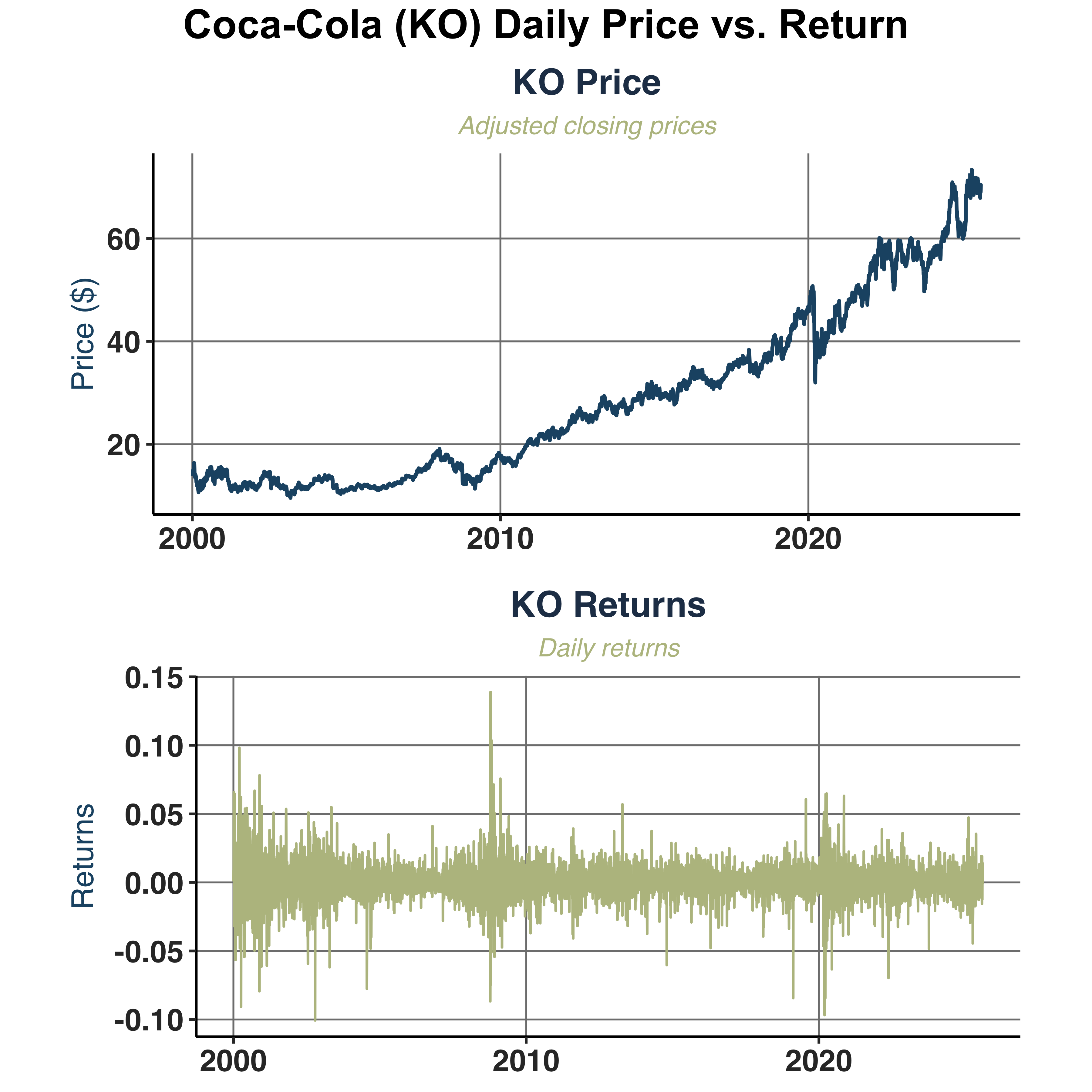
Compare daily adjusted closing prices against daily returns of Coca-Cola (KO).
 1
 2
 3
 4
 5
 6
 7
 8
 9
10
11
12
13
14
15
16
17
|
# Extract Coca-Cola (KO)
KO_daily <- filter(daily_returns, symbol == "KO")
KO_weekly <- filter(weekly_returns, symbol == "KO")
KO_monthly <- filter(monthly_returns, symbol == "KO")

price_return_plt <- plot_price_return(KO_daily, ticker_name = "KO",
                    save_pdf = TRUE, filename = "Plots/KO_Price_Return",
                    plot_width = 6, plot_height = 4)
combined_chart <- price_return_plt$combined
# Add grand title
combined_chart <- annotate_figure(combined_chart,
                                  top = text_grob("Coca-Cola (KO) Daily Price vs. Return",
                                                  color = "black",
                                                  face = "bold",
                                                  size = 16))

combined_chart
|
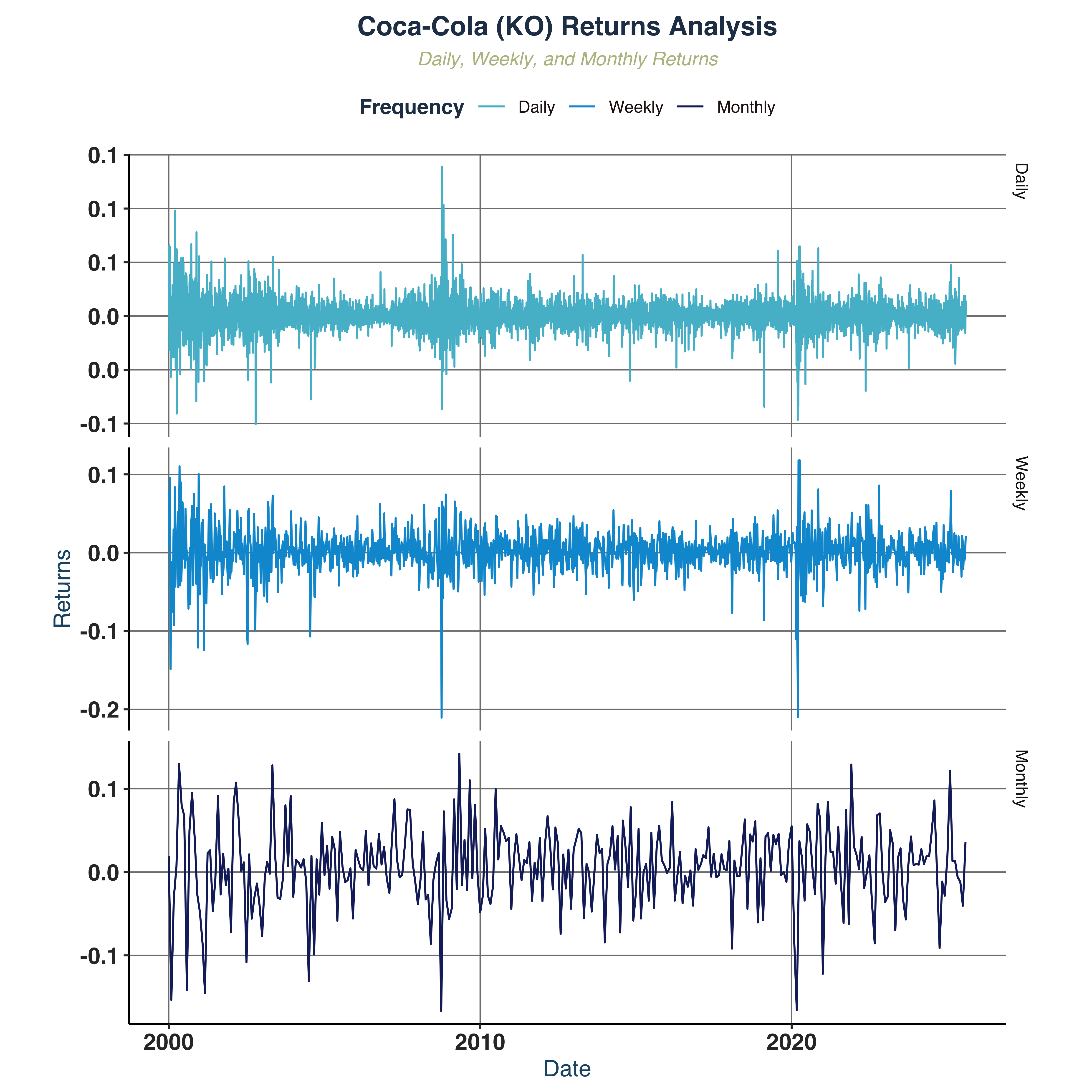
Compare returns across frequencies.
 1
 2
 3
 4
 5
 6
 7
 8
 9
10
11
12
13
14
15
16
17
18
19
20
21
22
23
24
25
26
27
28
29
30
31
32
|
# Combined plotting data
return_plot_dt <- rbind(
    select(KO_daily, c("date", "ret")) %>% mutate(freq="Daily"),
    select(KO_weekly, c("date", "ret")) %>% mutate(freq="Weekly"),
    select(KO_monthly, c("date", "ret")) %>% mutate(freq="Monthly")
  ) %>%
  mutate(freq = factor(freq, levels = c("Daily", "Weekly", "Monthly")))


# Line plot
returns_freq_plt <- return_plot_dt %>%
  ggplot(aes(x = date, y = ret, colour = freq)) +
  geom_line(size = 0.5) +
  scale_color_manual(values = c("Daily" = "#54BCD1FF",
                                "Weekly" = "#0099D5FF",
                                "Monthly" = "#172869FF")) +
  scale_y_continuous(labels = comma_format(accuracy = 0.1)) +
  facet_grid(freq ~ ., scales = "free_y") +
  labs(
    title = "Coca-Cola (KO) Returns Analysis",
    subtitle = "Daily, Weekly, and Monthly Returns",
    x = "Date",
    y = "Returns",
    color = "Frequency"
  ) +
  global_fonts

# Save with appropriate dimensions for vertical layout
ggsave("Plots/KO_Returns_By_Frequencies.pdf", returns_freq_plt,
       width = 8, height = 6, dpi = 300)

returns_freq_plt
|
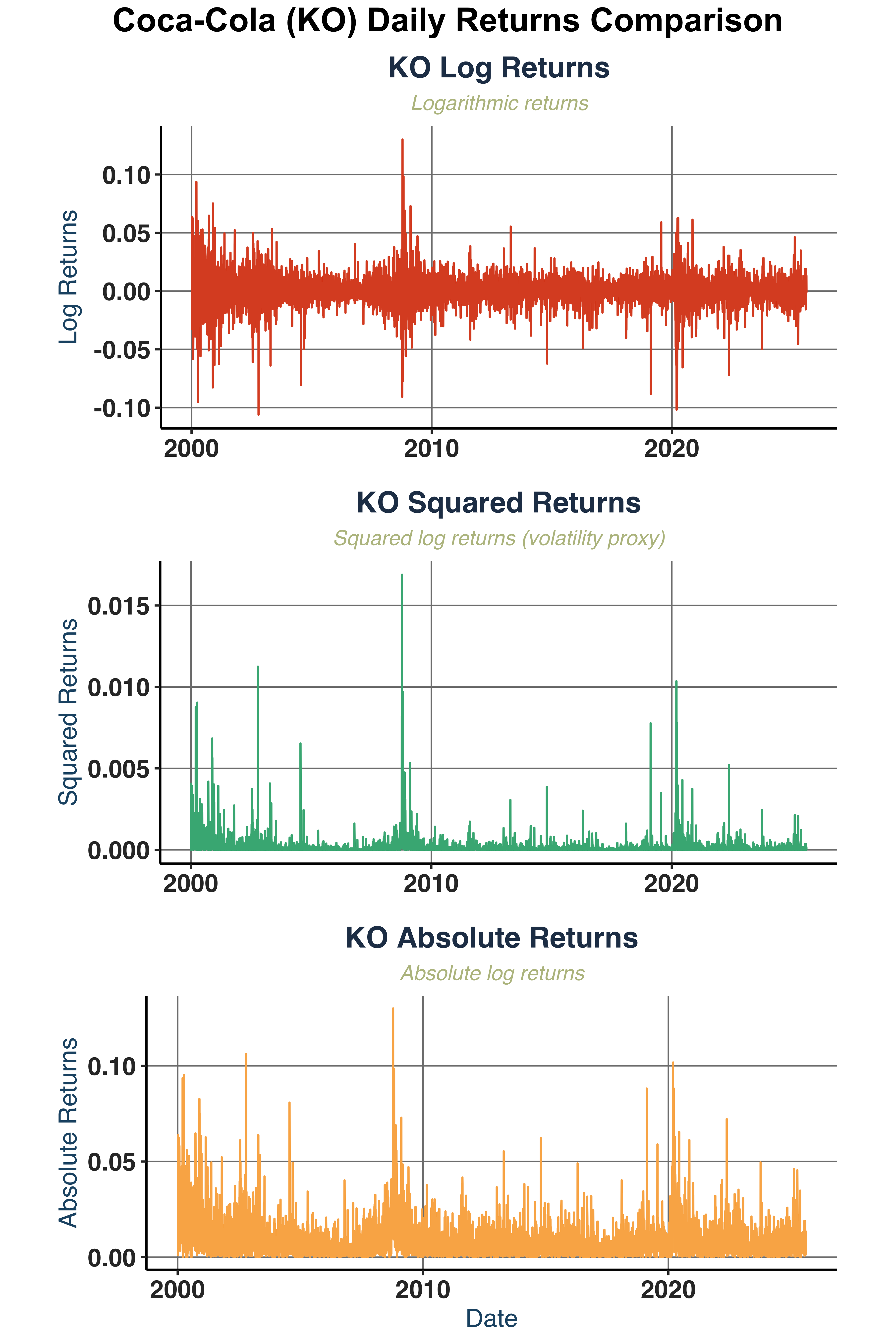
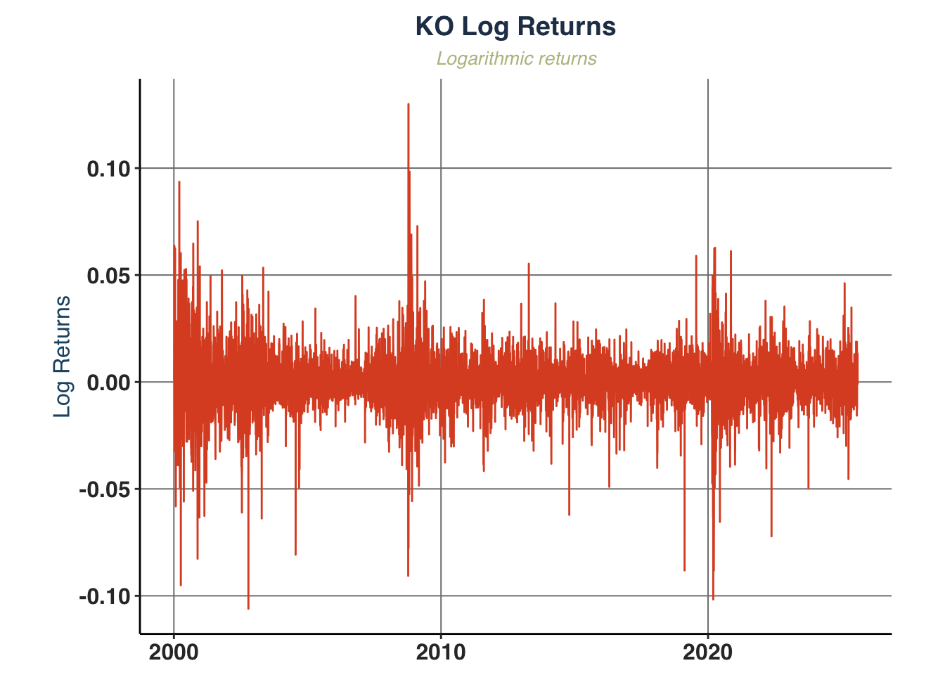
Plot log returns, squared returns, and absolute returns.
 1
 2
 3
 4
 5
 6
 7
 8
 9
10
11
12
|
daily_ret_plot <- plot_return_derivatives(
  KO_daily, ticker_name = "KO",
  save_pdf = TRUE, filename = "Plots/KO_daily_return_derivatives",
  plot_width = 6, plot_height = 3)
daily_ret_combined <- daily_ret_plot$combined
daily_ret_combined <- annotate_figure(daily_ret_combined ,
                                      top = text_grob("Coca-Cola (KO) Daily Returns Comparison",
                                                      color = "black",
                                                      face = "bold",
                                                      size = 16))

daily_ret_combined
|
1
2
3
|
# Note:
# We can apply the same logic and plot for weekly & monthly frequencies but I feel
# it's a bit abundant here. Thus, I only focus on daily basis analysis
|
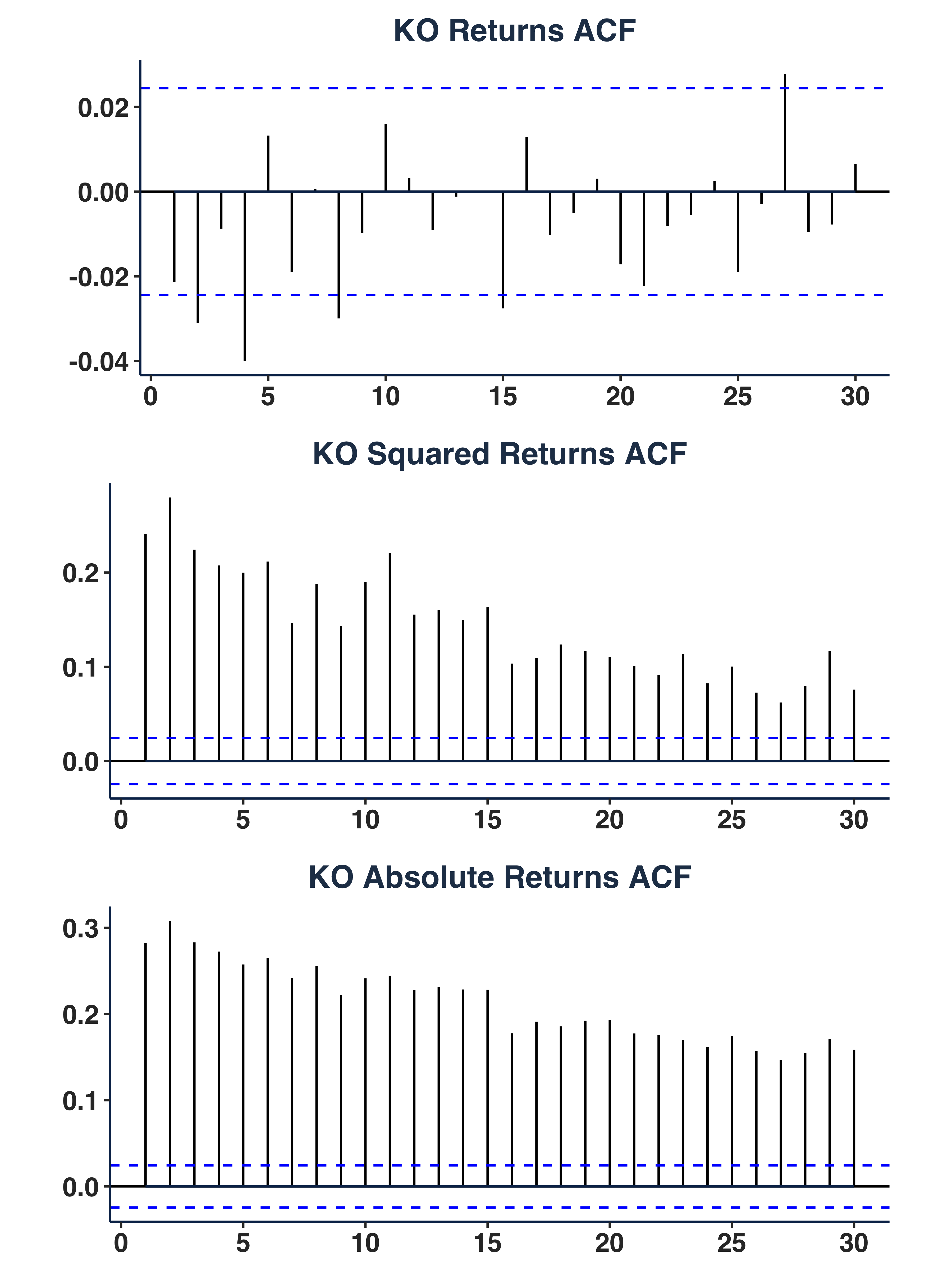
Plot autocorrelation function.
1
2
3
4
5
6
7
8
|
ret_acf_plots <- plot_acf_series(data = KO_daily,
                                 ticker_name = "KO",
                                 lag = 30,
                                 save_pdf = TRUE,
                                 filename = "Plots/ACF_Plots",
                                 plot_width = 6,
                                 plot_height = 3)
ret_acf_plots$combined_plot
|
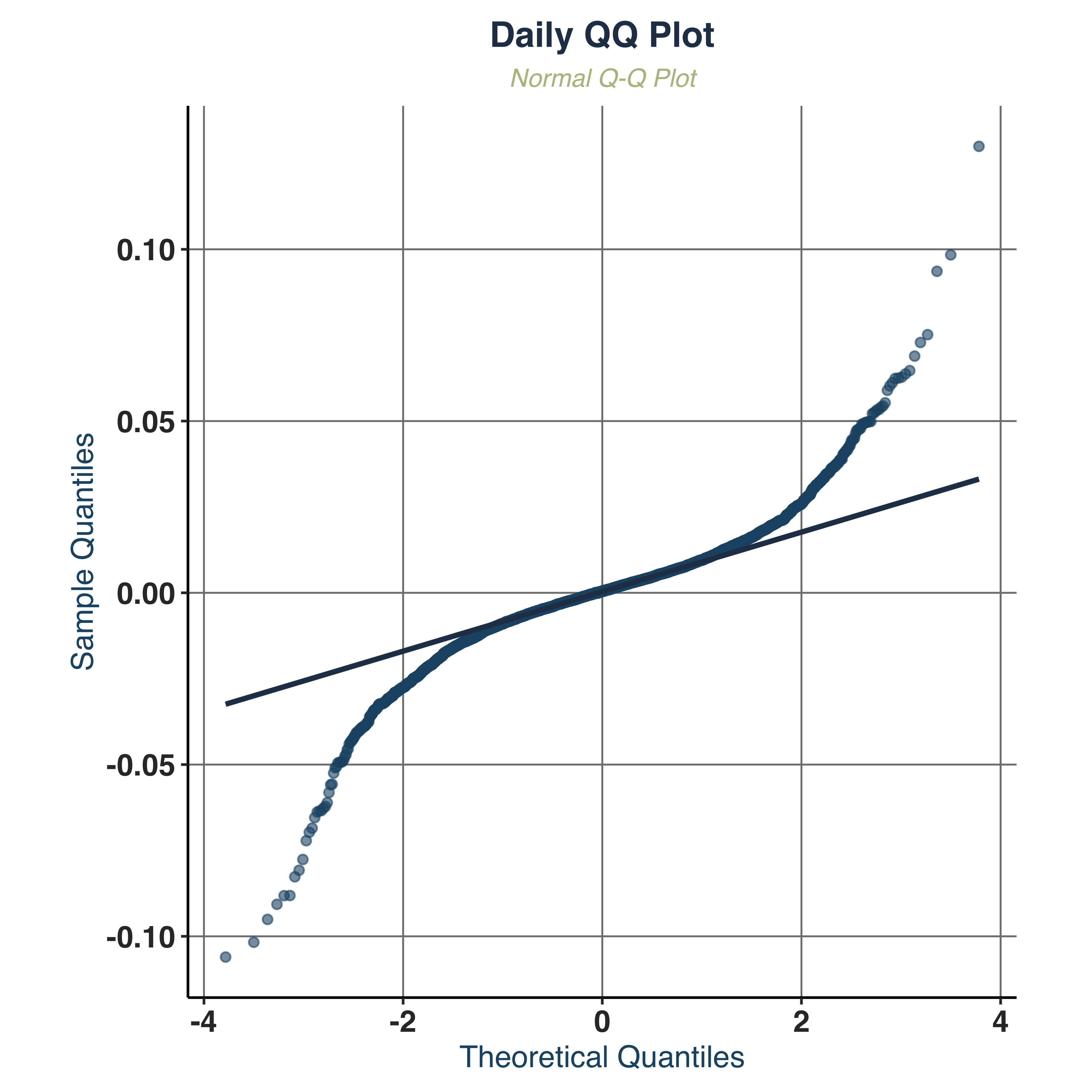
Examine QQ-Plot.
1
2
3
4
5
|
qq_plt <- qq_plot(KO_daily, KO_weekly, KO_monthly,
        ticker_name = "KO", save_pdf = TRUE,
        filename = "Plots/KO_QQ_Plot",
        plot_width = 4, plot_height = 4)
qq_plt$daily
|
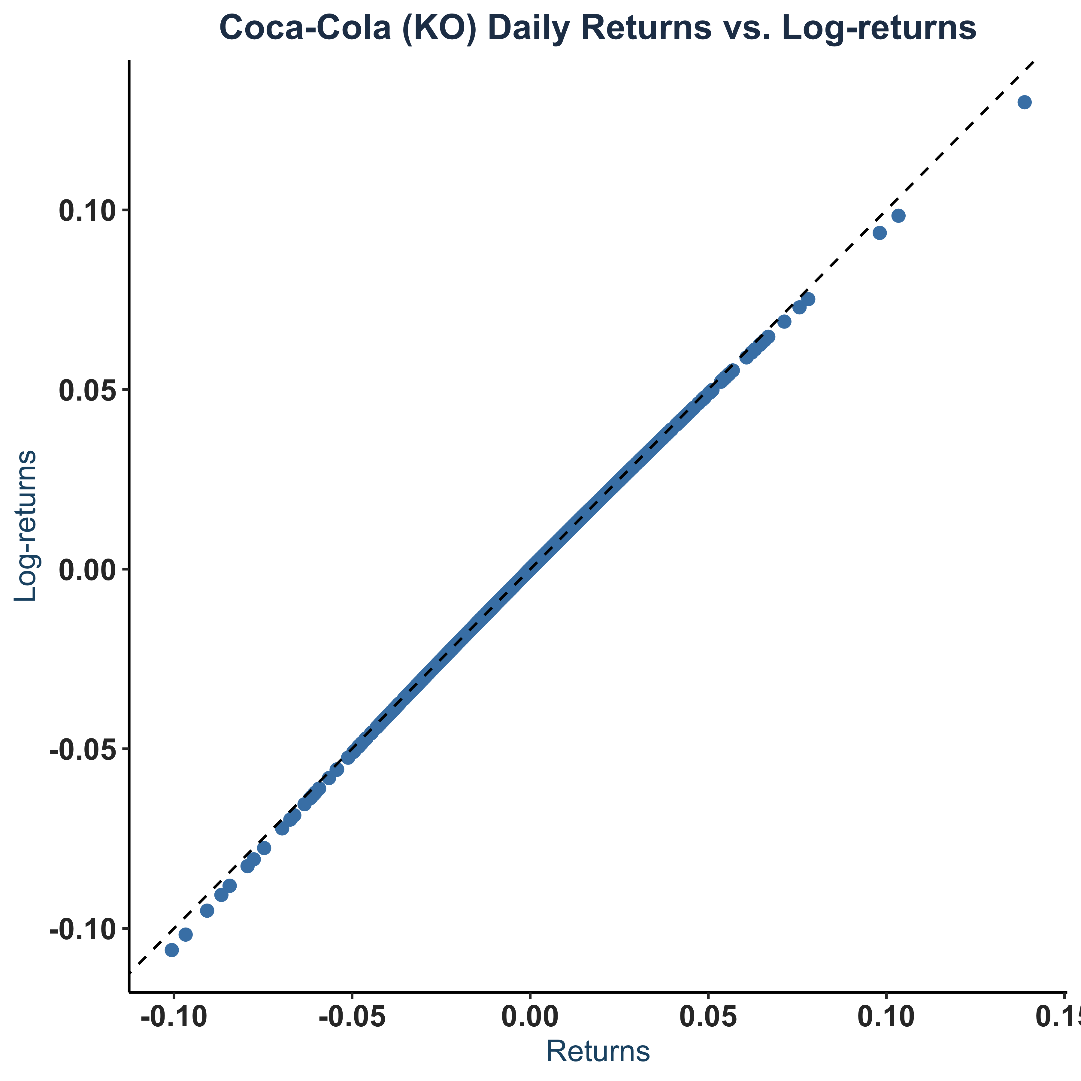
Scatter Plot of returns vs log-returns.
 1
 2
 3
 4
 5
 6
 7
 8
 9
10
11
12
13
14
15
16
17
18
19
20
21
22
|
sct_plt <- KO_daily |>
  ggplot(aes(x = ret, y = logret)) +
  geom_point(color = "steelblue",size=2) +
  geom_abline(linetype="dashed") +
  theme_bw() +
  theme(axis.line = element_line(colour = "black"),
        panel.grid.major = element_blank(),
        panel.grid.minor = element_blank(),
        panel.border = element_blank(),
        panel.background = element_blank()) +
  labs(
    title = "Coca-Cola (KO) Daily Returns vs. Log-returns",
    x = "Returns",
    y = "Log-returns"
  )+
  global_fonts

# Save to pdf
pdf(paste0(c("Plots/KO_Returns_LogReturns_Daily.pdf"),collapse = ""),
    width=4, height=4)
dev.off()
sct_plt
|
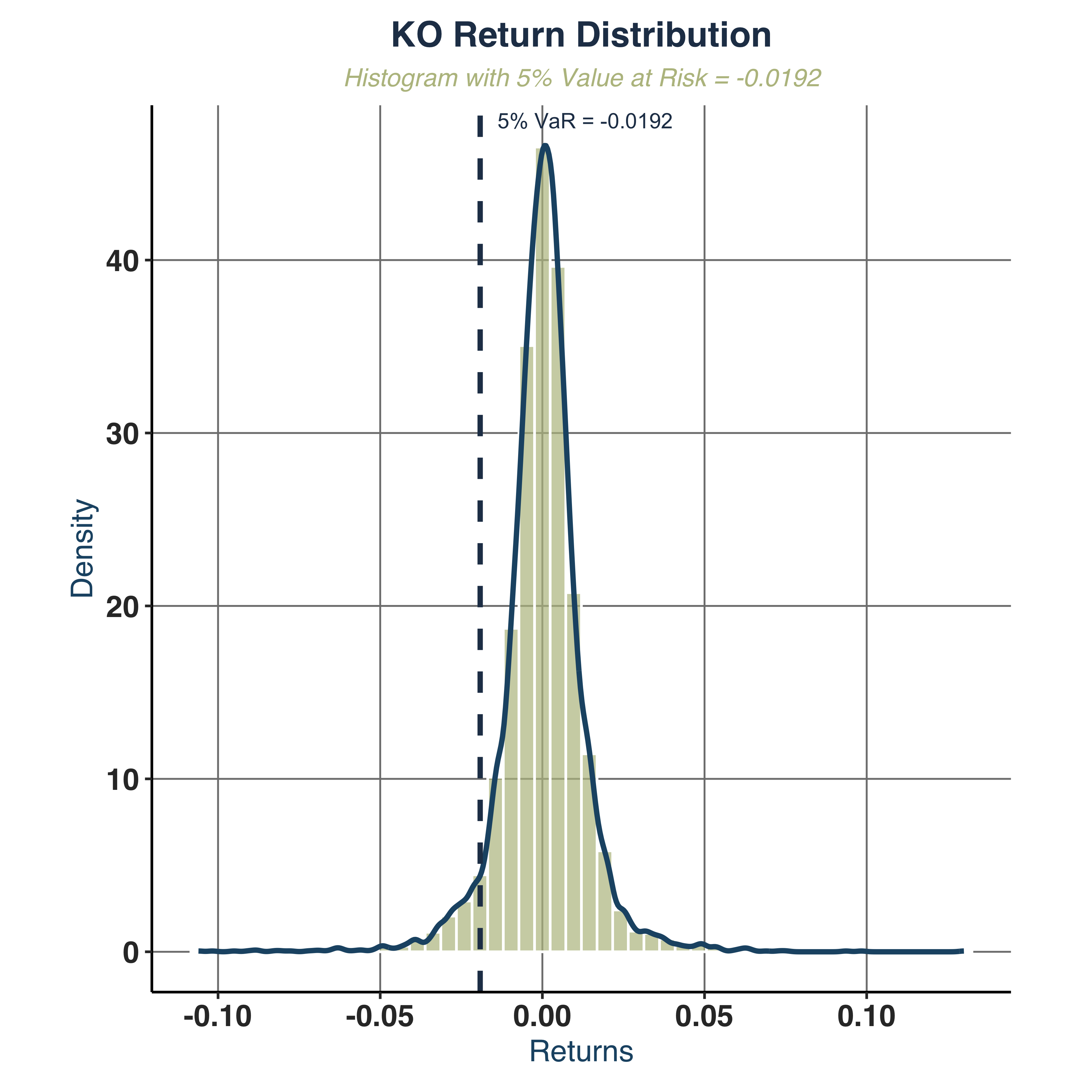
Plot histogram with 5% VaR.
1
2
3
4
|
hist_plt <- plot_histogram_var(KO_daily, ticker_name = "KO",
                               save_pdf = TRUE, filename = "Plots/KO_Histogram_Analysis",
                               confidence_level = 0.05)
hist_plt
|
1
2
3
4
|
##
## $var_5pct
##          5%
## -0.01917894
|
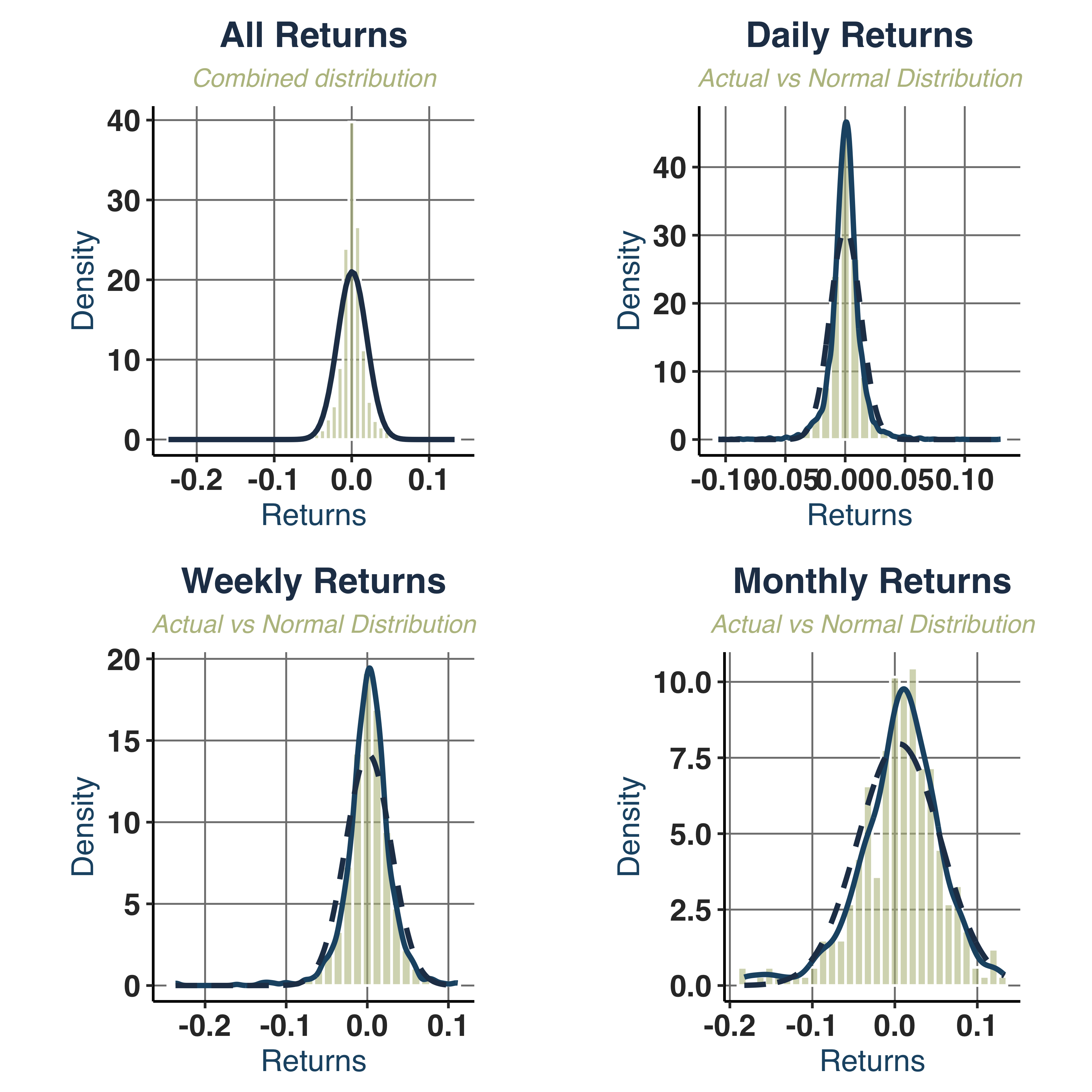
Create a normal distribution with same mean and standard deviation.
1
2
3
4
5
|
norm_dist_plt <- plot_normal_comparison(KO_daily, KO_weekly, KO_monthly,
                                        ticker_name = "KO", save_pdf = TRUE,
                                        filename = "Plots/KO_Normality_Test",
                                        plot_width = 8, plot_height = 6)
print(norm_dist_plt$combined)
|
iii. Analysis of GARCH Properties#
1. Return Distribution:
- Mean Reversion: returns fluctuate around zero mean (
mean=0.0004).
- Negative Skewness (
-0.37): left tail is heavier -> more extreme negative returns.
- Kurtosis (
16.43): fat tail, higher than normal from 7.7 to 13.4.
- Normality:
JB_PValue=0.0000 => strongly rejects normality across all frequencies.
2. Volatility Patterns:
- Volatility Clustering: visible in the returns series, showed in
Coca−Cola (KO) Daily Price vs. Return graph.
- Scale effect: higher frequencies magnify the volatility clustering effect, indicated in
Coca−Cola (KO) Returns Analysis graph.
3. Autocorrelation Structure:
- Returns ACF: fluctuate around `[-0.02, 0.02] -> no linear dependence.
- Squared/Absolute Returns ACF: significant autocorrelation (up to lag 30) -> GARCH effect.
4. Risk Characteristics:
- Value at Risk (VaR):
VaR_5pct range from -2.1% to -8.5%.
- Asymmetric Risk: more downside risks than upside potentials.
- Sharpe Ratio: poorly risk-adjusted performance (
Sharpe_Ratio<0.5 across all frequencies), but it is improved along with holding period.
b. Estimate Conditional Volatility Models#
i. Identify Model Specification#
First, we need to set up lower & upper bound for the model and test for ARCH effect on the squared (log-)returns.
 1
 2
 3
 4
 5
 6
 7
 8
 9
10
11
12
13
14
15
16
17
|
## 1. Setup Estimation Specs ----
# extract interested stock
# Extract log returns for KO
log_ret_real <- KO_daily$logret

ensembles <- 1
y <- matrix(log_ret_real, ncol = ensembles)

# Positivity of parameters and stationarity
lb.GARCH <- c(0.00000001, 0.00000001, 0,      0.00000001)
ub.GARCH <- c(0.2,        0.4,        0.9999, 0.9999)

# starting values: mu, omega, alpha, beta (not used directly in multi-start)
# b0      <- c(0, 0.0001, 0.2, 0.04)
## 2. Test for Model Specs
# i. Ljung-Box test on squared returns
Box.test(y^2, lag = 10, type = "Ljung-Box")
|
1
2
3
4
5
|
##
## 	Box-Ljung test
##
## data:  y^2
## X-squared = 2755.8, df = 10, p-value < 2.2e-16
|
1
2
|
# ii. ARCH test
ArchTest(y^2, lags = 5)
|
1
2
3
4
5
|
##
## 	ARCH LM-test; Null hypothesis: no ARCH effects
##
## data:  y^2
## Chi-squared = 225.68, df = 5, p-value < 2.2e-16
|
1
2
3
4
5
6
7
|
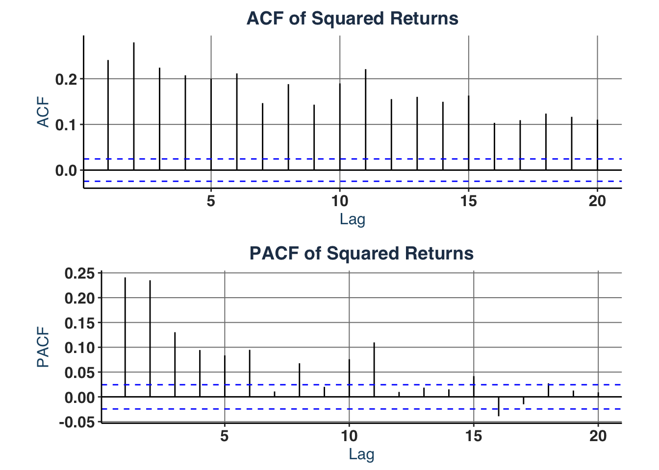
# iii. Partial- & Autocorrelation in squared returns (suggests GARCH order)
acf_plt <- ggAcf(y^2, lag.max = 20) +
  labs(title = "ACF of Squared Returns")
pacf_plt <- ggPacf(y^2, lag.max = 20) +
  labs(title = "PACF of Squared Returns")
acfs_plt <- ggarrange(acf_plt, pacf_plt, nrow = 2)
acfs_plt
|
1
2
|
# iv. Basic statistics
cat("Skewness:", moments::skewness(y^2), "\n")
|
1
|
cat("Kurtosis:", moments::kurtosis(y^2), "\n")
|
It shows that GARCH(1,1) (base model), GARCH(2,1), or GARCH(3,1) specifications are suitable for the estimate as:
- ACF shows slow, gradual decay -> GARCH term order 1 ($q = 1$).
- PACF shows sharp cutoff after lag 2, but lag 3 is still significant -> ARCH term order 1-3 ($p \in [1,3]$).
We can use GARCH(1,1) model as benchmark for Likelihood Ratio test, even for comparison with other extensions (e.g. GJR-GARCH).
Now, we estimate the base model sGARCH(1,1):
 1
 2
 3
 4
 5
 6
 7
 8
 9
10
11
12
13
14
15
16
17
18
19
20
21
22
23
24
25
26
27
28
29
30
31
32
33
34
|
## 3. Estimate GARCH (Multi-Start) ----
control.solnp <- list( rho        = 1,
                       # penalty weighting scalar for infeasibility in the
                       # augmented objective function: default is 1
                       outer.iter = 600,
                       # Maximum number of major (outer) iterations (default 400).
                       inner.iter = 800,
                       # Maximum number of minor (inner) iterations (default 800).
                       delta      = 1e-7,
                       # Relative step size in forward difference evaluation (default 1.0e-7).
                       tol        = 1e-6)

set.seed(1340) # for reproducibility

if (!file.exists("Data/KO_GARCH_base_mdl.rds")) {
  base_mdl <- estimate_garch_dynamic(
    y = y,
    n_starts = 10, # change number of random starts here, better set to 100
    garch_order = c(1,1),
    model_type = "sGARCH", # choose model
    distribution = "norm", # choose error distribution
    lower_bounds = lb.GARCH,
    upper_bounds = ub.GARCH,
    loglik_func = Likelihood.GARCH,
    ineq_constraints = Inequality.constraints.GARCH,
    custom_control = control.solnp
  )

  # Save results
  saveRDS(base_mdl, file = "Data/KO_GARCH_base_mdl.rds")
} else {
  # Access saved  data
  base_mdl <- readRDS("Data/KO_GARCH_base_mdl.rds")
}
|
1
2
3
4
|
## 4. Display Result ----
# Print best SOLNP results
stock_name <- "KO"
head(base_mdl$best_estimates$solnp, -1)
|
1
2
|
##            mu         omega         alpha          beta
## -2.315184e-06  8.401866e-05  5.516400e-02  9.429768e-01
|
1
2
3
4
|
best_solnp_loglik <- base_mdl$best_estimates$solnp["LogL"]

# Print best rugarch results
head(base_mdl$best_estimates$rugarch, -1)
|
1
2
3
4
5
6
|
##              mu           omega           alpha            beta           se_mu
##    4.733879e-04    1.631421e-06    5.825871e-02    9.312543e-01    1.190809e-04
##        se_omega        se_alpha         se_beta    se_robust_mu se_robust_omega
##             NaN             NaN             NaN    2.845166e-04    2.029449e-05
## se_robust_alpha  se_robust_beta
##    2.484959e-01    2.635755e-01
|
1
|
best_rugarch_loglik <- base_mdl$best_estimates$rugarch["LogL"]
|
Then, we estimate higher-order model sGARCH(2,1):
 1
 2
 3
 4
 5
 6
 7
 8
 9
10
11
12
13
14
15
16
17
18
19
20
21
22
23
24
25
|
# Set bounds for GARCH-N
lw_bs <- c(-0.05, 1e-08, 1e-06, 1e-06, 1e-6)  # [mu, omega, alpha1, beta1, beta2]
up_bs <- c(0.1,   0.3,  0.2, 0.2, 0.85) # [mu, omega, alpha1, beta1, beta2]

if (!file.exists("Data/KO_GARCH_sg21_mdl.rds")) {
  ## 5. Re-estimate GARCH (Multi-Start) ----
  sg21_mdl <- estimate_garch_dynamic(
    y = y,
    n_starts = 10, # change number of random starts here, better set to 100
    garch_order = c(2,1),
    model_type = "sGARCH", # choose model
    distribution = "norm", # choose error distribution
    lower_bounds = lw_bs,
    upper_bounds = up_bs,
    loglik_func = Likelihood.GARCH,
    ineq_constraints = Inequality.constraints.GARCH,
    custom_control = control.solnp
  )

  # Save results
  saveRDS(sg21_mdl, file = "Data/KO_GARCH_sg21_mdl.rds")
} else {
  # Access saved  data
  sg21_mdl <- readRDS("Data/KO_GARCH_sg21_mdl.rds")
}
|
1
2
3
4
5
|
# Find best fits
best_solnp_idx   <- which.max(sg21_mdl$solnp_results[, "LogL"])
best_rugarch_idx <- which.max(sg21_mdl$rugarch_results[, "LogL"])
# Print best SOLNP results
head(sg21_mdl$best_estimates$solnp, -1)
|
1
2
|
##           mu        omega       alpha1       alpha2         beta
## 6.781344e-04 9.122594e-05 1.730226e-01 1.092850e-01 1.092859e-01
|
1
2
3
4
|
sg21_best_solnp_loglik <- sg21_mdl$best_estimates$solnp["LogL"]

# Print best rugarch results
head(sg21_mdl$best_estimates$rugarch, -1)
|
1
2
3
4
5
6
7
8
|
##               mu            omega           alpha1           alpha2
##     4.781701e-04     1.624803e-06     5.840805e-02     4.891468e-08
##             beta            se_mu         se_omega        se_alpha1
##     9.311935e-01     1.197180e-04              NaN     1.117900e-02
##        se_alpha2          se_beta     se_robust_mu  se_robust_omega
##     5.959924e-03              NaN     1.369747e-04     3.679863e-06
## se_robust_alpha1 se_robust_alpha2   se_robust_beta
##     2.758160e-02     8.551859e-02     6.484744e-02
|
1
|
sg21_best_rugarch_loglik <- sg21_mdl$best_estimates$rugarch["LogL"]
|
1
2
3
4
5
6
7
8
9
|
ll_restricted <- best_solnp_loglik        # GARCH(1,1)
ll_unrestricted <- sg21_best_solnp_loglik # GARCH(2,1)
p_restricted <- 4            # Number of parameters in restricted model
p_unrestricted <- 5          # Number of parameters in unrestricted model

# LRT
lr_stat <- 2 * (ll_unrestricted - ll_restricted)
p_value <- 1 - pchisq(lr_stat, p_unrestricted - p_restricted)
cat("LR =", round(lr_stat, 3), ", p =", round(p_value, 4), ", Decision:", ifelse(p_value < 0.05, "REJECT H0 (unrestricted better)", "FAIL TO REJECT H0 (restricted adequate)"), "\n")
|
1
|
## LR = -9911.39 , p = 1 , Decision: FAIL TO REJECT H0 (restricted adequate)
|
The LRT implies that simpler model provide a better estimate for our dataset, hence we will apply this specification for the estimate of required models: GARCH-N, GARCH-t, EGARCH and GJR-GARCH-N.
ii. GARCH-N Estimate#
 1
 2
 3
 4
 5
 6
 7
 8
 9
10
11
12
13
14
15
16
17
18
19
20
|
if (!file.exists("Data/KO_GARCH_gn_mdl.rds")) {
  gn_mdl <- estimate_garch_dynamic(
    y = y,
    n_starts = 10, # change number of random starts here, better set to 100
    garch_order = c(1,1),
    model_type = "GARCH-N", # choose model
    distribution = "norm", # choose error distribution
    lower_bounds = lb.GARCH,
    upper_bounds = ub.GARCH,
    loglik_func = Likelihood.GARCH,
    ineq_constraints = Inequality.constraints.GARCH,
    custom_control = control.solnp
  )

  # Save results
  saveRDS(gn_mdl, file = "Data/KO_GARCH_gn_mdl.rds")
} else {
  # Access saved  data
  gn_mdl <- readRDS("Data/KO_GARCH_gn_mdl.rds")
}
|
1
2
3
4
|
# Extract best parameter estimate & best fit model
gn_best_fit <- gn_mdl$best_models
gn_best_rugarch_pars <- head(gn_mdl$best_estimates$solnp,-1)
gn_best_rugarch_pars
|
iii. GARCH-t Estimate#
 1
 2
 3
 4
 5
 6
 7
 8
 9
10
11
12
13
14
15
16
17
18
19
20
21
22
23
24
25
26
27
28
29
30
|
# GARCH-t bounds
# Parameter order: [mu, omega, alpha1, beta1, nu]
lwb <- c(-0.1,   1e-6,  1e-6,  1e-6,  2.1)
upb <- c( 0.1,   0.1,   0.3,   0.95,  30.0)

if (!file.exists("Data/KO_GARCH_gt_mdl.rds")) {
  gt_mdl <- estimate_garch_dynamic(
    y = y,
    n_starts = 10, # change number of random starts here, better set to 100
    garch_order = c(1,1),
    model_type = "GARCH-t", # choose model
    distribution = "norm", # choose error distribution
    lower_bounds = lwb,
    upper_bounds = upb,
    loglik_func = Likelihood.GARCH,
    ineq_constraints = Inequality.constraints.GARCH,
    custom_control = control.solnp
  )

  # Save results
  saveRDS(gt_mdl, file = "Data/KO_GARCH_gt_mdl.rds")
} else {
  # Access saved  data
  gt_mdl <- readRDS("Data/KO_GARCH_gt_mdl.rds")
}

# Extract model data
gt_best_fit <- gt_mdl$best_models
gt_best_rugarch_pars <- gt_mdl$best_estimates$rugarch[1:5]
gt_best_rugarch_pars
|
iv. EGARCH Estimate#
 1
 2
 3
 4
 5
 6
 7
 8
 9
10
11
12
13
14
15
16
17
18
19
20
21
22
23
24
25
26
27
28
29
30
|
# EGARCH Bounds
# Parameter order: [mu, omega, alpha1, gamma1, beta1]
eg_lb <- c(-0.1,  -2.0,  -1.0,  -1.0,  -0.99)
eg_up <- c( 0.1,   0.5,   1.0,   1.0,   0.99)

if (!file.exists("Data/KO_GARCH_eg_mdl.rds")) {
  eg_mdl <- estimate_garch_dynamic(
    y = y,
    n_starts = 10, # change number of random starts here, better set to 100
    garch_order = c(1,1),
    model_type = "EGARCH", # choose model
    distribution = "norm", # choose error distribution
    lower_bounds = eg_lb,
    upper_bounds = eg_up,
    loglik_func = Likelihood.GARCH,
    ineq_constraints = Inequality.constraints.GARCH,
    custom_control = control.solnp
)

  # Save results
  saveRDS(eg_mdl, file = "Data/KO_GARCH_eg_mdl.rds")
} else {
  # Access saved  data
  eg_mdl <- readRDS("Data/KO_GARCH_eg_mdl.rds")
}

# Extract model data
eg_best_fit <- eg_mdl$best_models
eg_best_rugarch_pars <- eg_mdl$best_estimates$rugarch[1:5]
eg_best_rugarch_pars
|
v. GJR-GARCH-N Estimate#
 1
 2
 3
 4
 5
 6
 7
 8
 9
10
11
12
13
14
15
16
17
18
19
20
21
22
23
24
25
26
27
28
29
30
|
# GJR-GARCH-N bounds
# Parameter order: [mu, omega, alpha1, gamma1, beta1]
gjr_lb <- c(-0.1,   1e-6,  1e-6,  1e-6,  1e-6)
gjr_ub <- c( 0.1,   0.1,   0.3,   0.5,   0.95)

if (!file.exists("Data/KO_GARCH_gjrgn_mdl.rds")) {
  gjrgn_mdl <- estimate_garch_dynamic(
    y = y,
    n_starts = 10, # change number of random starts here, better set to 100
    garch_order = c(1,1),
    model_type = "GJR-GARCH-N", # choose model
    distribution = "norm", # choose error distribution
    lower_bounds = gjr_lb,
    upper_bounds = gjr_ub,
    loglik_func = Likelihood.GARCH,
    ineq_constraints = Inequality.constraints.GARCH,
    custom_control = control.solnp
  )

  # Save results
  saveRDS(gjrgn_mdl, file = "Data/KO_GARCH_gjrgn_mdl.rds")
} else {
  # Access saved  data
  gjrgn_mdl <- readRDS("Data/KO_GARCH_gjrgn_mdl.rds")
}

# Extract model data
gjrgn_best_fit <- gjrgn_mdl$best_models
gjrgn_best_rugarch_pars <- gjrgn_mdl$best_estimates$rugarch[1:5]
gjrgn_best_rugarch_pars
|
vi. Result Comparison & Plots#
 1
 2
 3
 4
 5
 6
 7
 8
 9
10
11
12
13
14
15
16
17
18
19
20
21
22
23
24
25
26
27
28
29
30
31
32
33
34
|
# Get all unique parameter names
all_params <- unique(c(
  names(gn_best_rugarch_pars),
  names(gt_best_rugarch_pars),
  names(eg_best_rugarch_pars),
  names(gjrgn_best_rugarch_pars)
))

# Create empty matrix
results_matrix <- matrix(NA, nrow = 4, ncol = length(all_params))
rownames(results_matrix) <- c("GARCH-N", "GARCH-t", "EGARCH", "GJR-GARCH-N")
colnames(results_matrix) <- all_params

# Fill in the values
for (param in names(gn_best_rugarch_pars)) {
  results_matrix["GARCH-N", param] <- gn_best_rugarch_pars[param]
}

for (param in names(gt_best_rugarch_pars)) {
  results_matrix["GARCH-t", param] <- gt_best_rugarch_pars[param]
}

for (param in names(eg_best_rugarch_pars)) {
  results_matrix["EGARCH", param] <- eg_best_rugarch_pars[param]
}

for (param in names(gjrgn_best_rugarch_pars)) {
  results_matrix["GJR-GARCH-N", param] <- gjrgn_best_rugarch_pars[param]
}

# Convert to data frame
results_df <- as.data.frame(results_matrix)
names(results_df)[names(results_df) == "shape"] <- "nu"
print((results_df))
|
 1
 2
 3
 4
 5
 6
 7
 8
 9
10
|
##                       mu         omega       alpha      beta       nu
## GARCH-N     0.0002967198  7.560890e-05  0.12667254 0.8233275       NA
## GARCH-t     0.0004948997  1.533138e-06  0.06400793 0.9266939 4.973822
## EGARCH      0.0002579436 -1.158257e-01 -0.04981127 0.9863477       NA
## GJR-GARCH-N 0.0003411014  1.688795e-06  0.02709499 0.9307542       NA
##                  gamma
## GARCH-N             NA
## GARCH-t             NA
## EGARCH      0.12945606
## GJR-GARCH-N 0.06202623
|
1
2
3
4
|
log_ret_plot <- plot_return_derivatives(
  KO_daily, ticker_name = "KO",
  plot_width = 6, plot_height = 3)
log_ret_plot$logret
|
 1
 2
 3
 4
 5
 6
 7
 8
 9
10
11
12
13
14
15
16
17
18
19
20
21
22
23
24
25
26
27
28
29
30
31
32
33
34
35
36
37
38
39
40
41
42
43
44
45
|
## Simulate series for estimated models
# Get number observations
T_obs <- length(log_ret_real)
# Create matrix of sigma values across models
sig_KO <- cbind(
rugarch::sigma(gn_best_fit$rugarch),
rugarch::sigma(gt_best_fit$rugarch),
rugarch::sigma(eg_best_fit$rugarch),
rugarch::sigma(gjrgn_best_fit$rugarch)
)
colnames(sig_KO) <- c("GARCH-N", "GARCH-t", "EGARCH", "GJR-GARCH-N")
# Create plot data
plot_data <- cbind("Squared Returns" = KO_daily$sqret, sig_KO)
# Create time series object with actual dates
ts_data <- ts(plot_data,
start = c(year(min(KO_daily$date)), yday(min(KO_daily$date))),
frequency = 365.25)
# Plot all series
colors <- c("Squared.Returns" = "gray40",
"GARCH.N" = "#663171FF",
"GARCH.t" = "#EA7428FF",
"EGARCH" = "#0C7156FF",
"GJR.GARCH.N" = "#3A507FFF")
sim_plot <- autoplot(ts_data) +
scale_color_manual(values = colors)+
theme(axis.line = element_line(colour = "black"),
panel.grid.major = element_blank(),
panel.grid.minor = element_blank(),
panel.border = element_blank(),
panel.background = element_blank(),
legend.position = "bottom"
) +
global_fonts+
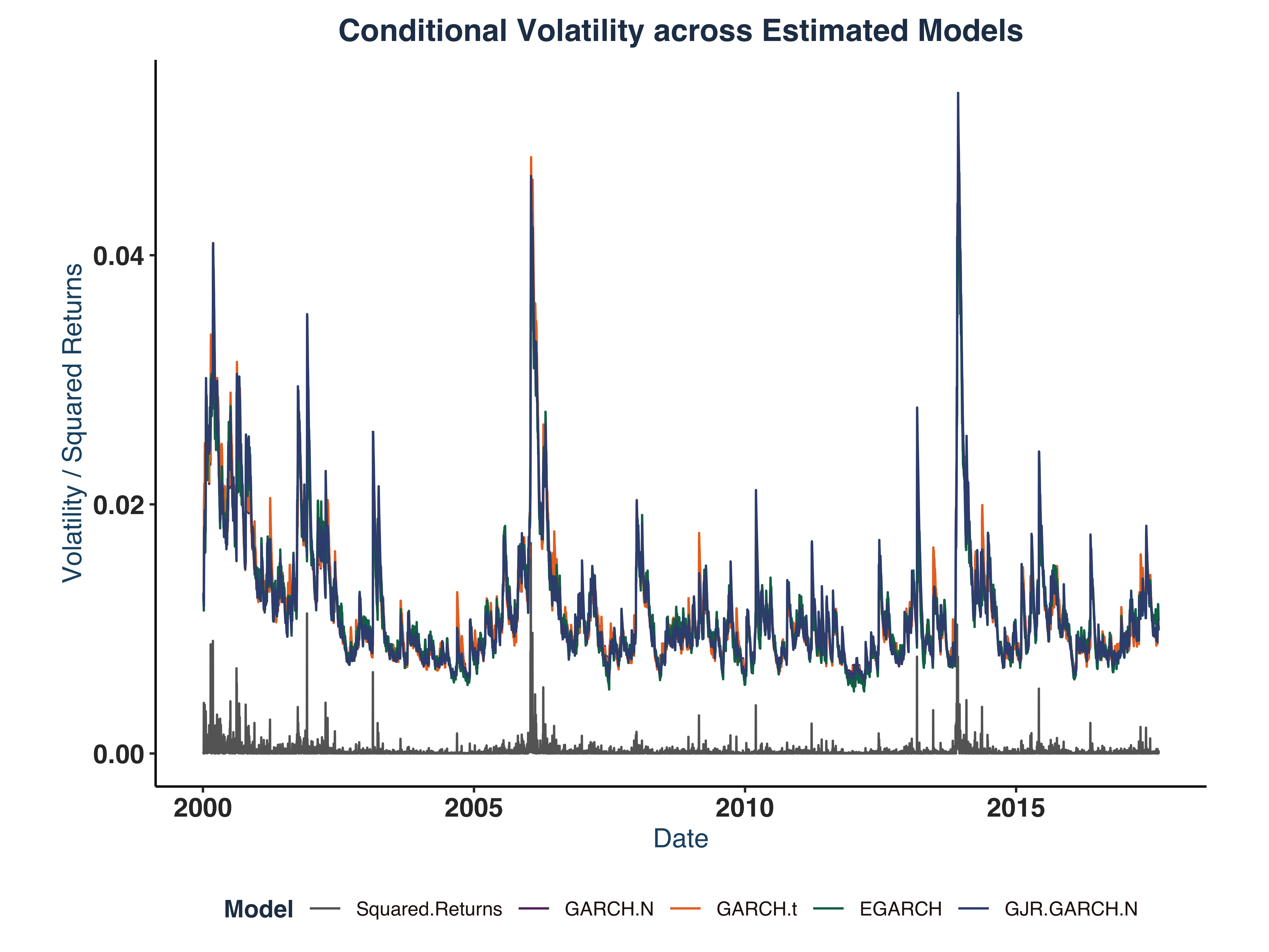
labs(
title = "Conditional Volatility across Estimated Models",
x = "Date",
y = "Volatility / Squared Returns",
color = "Model"
)
print(sim_plot)
|
vii. Evidence of Excessive Kurtosis & Skewness#
 1
 2
 3
 4
 5
 6
 7
 8
 9
10
11
12
13
14
15
16
17
18
19
20
21
22
23
24
25
26
27
28
29
30
|
# Extact standardized residuals
std_resid_gn <- rugarch::residuals(gn_best_fit$rugarch, standardize = TRUE)
std_resid_gt <- rugarch::residuals(gt_best_fit$rugarch, standardize = TRUE)
std_resid_eg <- rugarch::residuals(eg_best_fit$rugarch, standardize = TRUE)
std_resid_gjr <- rugarch::residuals(gjrgn_best_fit$rugarch, standardize = TRUE)

# Helper function to extract test result
get_jb_results <- function(residuals) {
  jb_test <- jarque.bera.test(residuals)
  return(c(
    JB_Statistic = as.numeric(jb_test$statistic),
    JB_p_value = as.numeric(jb_test$p.value)
  ))
}

# Create the residuals list
residuals_list <- list(std_resid_gn, std_resid_gt, std_resid_eg, std_resid_gjr)

# Create the data frame of kurtosis, excess kurtosis, and test results
kurtosis_results <- data.frame(
  Model = c("GARCH-N", "GARCH-t", "EGARCH", "GJR-GARCH-N"),
  Kurtosis = c(kurtosis(std_resid_gn), kurtosis(std_resid_gt),
               kurtosis(std_resid_eg), kurtosis(std_resid_gjr)),
  Excess_Kurtosis = c(kurtosis(std_resid_gn)-3, kurtosis(std_resid_gt)-3,
                      kurtosis(std_resid_eg)-3, kurtosis(std_resid_gjr)-3),
  JB_Statistic = sapply(residuals_list, function(x) get_jb_results(x)[1]),
  JB_p_value = sapply(residuals_list, function(x) get_jb_results(x)[2])
)

print(kurtosis_results)
|
1
2
3
4
5
|
##         Model Kurtosis Excess_Kurtosis JB_Statistic JB_p_value
## 1     GARCH-N 8.590343        5.590343     8562.986          0
## 2     GARCH-t 8.721817        5.721817     8967.117          0
## 3      EGARCH 8.467178        5.467178     8187.392          0
## 4 GJR-GARCH-N 8.407663        5.407663     8027.130          0
|
 1
 2
 3
 4
 5
 6
 7
 8
 9
10
11
12
13
14
15
16
17
18
|
# Calculate skewness of volatility
skewness_results <- data.frame(
  Volatility_Skewness = apply(sig_KO, 2, skewness)
)

# Test statistical significance of skewness
skewness_tests <- apply(sig_KO, 2, function(x) {
  # Skewness test (H0: skewness = 0)
  n <- length(x)
  skew_stat <- skewness(x)
  se_skew <- sqrt(6/n)  # Standard error of skewness
  z_stat <- skew_stat / se_skew
  p_value <- 2 * (1 - pnorm(abs(z_stat)))
  return(c(skewness = skew_stat, z_statistic = z_stat, p_value = p_value))
})

skewness_test_results <- data.frame(t(skewness_tests))
print(skewness_test_results)
|
1
2
3
4
5
|
##             skewness z_statistic p_value
## GARCH-N     2.622833    85.91529       0
## GARCH-t     2.630862    86.17830       0
## EGARCH      2.410865    78.97192       0
## GJR-GARCH-N 2.613715    85.61663       0
|
The test results show clear evidence of both excessive kurtosis and skewness in estimated models.
Moreover, it is clear that the highest volatility period is around 2013-2014, which seems to coincide with the declining soda consumption at the time.
c. Estimate 2.5% VaR & ES#
i. Estimation#
 1
 2
 3
 4
 5
 6
 7
 8
 9
10
11
12
13
14
15
16
17
18
19
20
21
22
23
24
|
# Specs Setup
n_IS    <- 4000           # no. simulation
alpha   <- 0.025          # 2.5% VaR
date_sr <- KO_daily$date  # Date labels

# Check if there exist saved model data
if (!file.exists("Data/KO_Residuals.rds")) {
  KO_res <- Estimate.VaR.ES.models(ret   = log_ret_real,
                                   alpha = alpha,
                                   n_IS  = n_IS,
                                   date  = date_sr)

  # Save model data
  saveRDS(KO_res, file = "Data/KO_Residuals.rds")
  # Extrac estimated dataset
  KO_qe_dt <- as.data.frame(KO_res$VaR.ES.df)
} else {
  # Access saved model data
  KO_res   <- readRDS("Data/KO_Residuals.rds")
  KO_qe_dt <- as.data.frame(KO_res$VaR.ES.df)
}

# Print some observations
tail(KO_qe_dt,5)
|
 1
 2
 3
 4
 5
 6
 7
 8
 9
10
11
12
13
14
15
16
17
18
19
20
21
22
23
24
25
26
27
28
29
30
|
##            date        ret q_GARCH_N e_GARCH_N hit_GARCH_N q_GARCH_t e_GARCH_t
## 2434 2025-08-04  0.1451146 -2.143210 -2.556375       FALSE -2.088496 -2.491113
## 2435 2025-08-05  0.1304311 -2.073038 -2.472675       FALSE -2.033012 -2.424932
## 2436 2025-08-06  0.6639734 -2.006067 -2.392793       FALSE -1.979413 -2.361001
## 2437 2025-08-07  1.3148655 -1.971980 -2.352136       FALSE -1.952074 -2.328392
## 2438 2025-08-08 -0.1278738 -2.028638 -2.419716       FALSE -1.998845 -2.384179
##      hit_GARCH_t q_GJRGARCH_t e_GJRGARCH_t hit_GJRGARCH_t q_RiskMetrics
## 2434       FALSE    -2.111282    -2.518292          FALSE     -2.003095
## 2435       FALSE    -2.048532    -2.443445          FALSE     -1.943322
## 2436       FALSE    -1.988499    -2.371839          FALSE     -1.885161
## 2437       FALSE    -1.941655    -2.315965          FALSE     -1.855321
## 2438       FALSE    -1.929409    -2.301357          FALSE     -1.906349
##      e_RiskMetrics hit_RiskMetrics q_HistSim e_HistSim hit_HistSim   q_GAS1F
## 2434     -2.389249           FALSE -2.050224 -2.706837       FALSE -1.721901
## 2435     -2.317953           FALSE -2.050224 -2.706837       FALSE -1.700777
## 2436     -2.248579           FALSE -2.050224 -2.706837       FALSE -1.680579
## 2437     -2.212986           FALSE -2.050224 -2.706837       FALSE -1.661259
## 2438     -2.273851           FALSE -2.050224 -2.706837       FALSE -1.642771
##        e_GAS1F hit_GAS1F   q_GAS2F   e_GAS2F hit_GAS2F  q_CAREAS  e_CAREAS
## 2434 -2.889322     FALSE -1.849358 -2.824393     FALSE -2.545021 -3.596716
## 2435 -2.853876     FALSE -1.819951 -2.796986     FALSE -2.294611 -3.346305
## 2436 -2.819985     FALSE -1.791847 -2.770399     FALSE -2.085626 -3.137320
## 2437 -2.787566     FALSE -1.764991 -2.744610     FALSE -1.956230 -3.007925
## 2438 -2.756544     FALSE -1.739330 -2.719597     FALSE -1.902551 -2.954245
##      hit_CAREAS q_CARESAV e_CARESAV hit_CARESAV   q_GAS_t   e_GAS_t hit_GAS_t
## 2434      FALSE -2.478974 -3.502481       FALSE -2.295290 -3.084985     FALSE
## 2435      FALSE -2.303023 -3.326529       FALSE -2.210291 -2.969971     FALSE
## 2436      FALSE -2.141791 -3.165298       FALSE -2.129779 -2.862278     FALSE
## 2437      FALSE -2.117940 -3.141447       FALSE -2.082508 -2.789670     FALSE
## 2438      FALSE -2.243956 -3.267463       FALSE -2.165320 -2.908771     FALSE
|
ii. VaR Analysis#
Estimated parameters:
 1
 2
 3
 4
 5
 6
 7
 8
 9
10
11
12
13
14
15
16
17
18
19
20
21
22
23
24
25
26
27
28
29
30
31
32
33
34
35
36
37
38
39
40
41
42
43
44
45
46
47
48
49
50
51
52
|
## Extract estimated parameters of interested models ----
# Declare list of models of interest
mdl_ls <- c("GARCH_N", "GJRGARCH_t", "CAREAS", "CARESAV", "GAS1F") # HistSim is non-parametric
# Model Names
mdl_names <- c("GARCH_N", "GJR_GARCH_t", "AS_CAViaR", "SAV_CAViaR", "GAS_1F")

# Assign empty result list
param_ests <- list()
# Extract estimated parameters
for (i in 1:length(mdl_ls)) {
  name <- mdl_names[i]
  model <- mdl_ls[i]

  param_ests[[name]] <- KO_res$pars[[model]]
}

## Print out results ----
# Define parameter structures for each model
param_structures <- list(
  "GARCH_N" = c("omega", "alpha1", "beta1"),
  "GJR_GARCH_t" = c("omega", "alpha1", "beta1", "gamma1", "shape"),
  "AS_CAViaR" = c("beta1", "beta2", "beta3", "beta4", "gamma1", "gamma2", "gamma3"),
  "SAV_CAViaR" = c("beta1", "beta2", "beta3", "gamma1", "gamma2", "gamma3"),
  "GAS_1F" = c("beta1", "gamma1", "alpha1", "alpha2")
)
# Get all unique parameter names
all_params <- unique(unlist(param_structures))

# Initialize a result table
param_tbl <- data.frame(Model=mdl_names, stringsAsFactors = FALSE)
for (param in all_params) {
  param_tbl[[param]] <- NA
}

# Fill in estimated parameters
for (model in mdl_names) {
  # Get row index
  row_id <- which(param_tbl$Model == model)

  # Get estimated parameters
  params <- c(param_ests[[model]]) # vectorise
  # Get corresponding names
  param_names <- param_structures[[model]]

  # Assign values
  for (i in 1:length(params)) {
    param_tbl[row_id, param_names[i]] <- params[i]
  }
}

names(param_tbl)[names(param_tbl) == "shape"] <- "nu"
print(param_tbl)
|
 1
 2
 3
 4
 5
 6
 7
 8
 9
10
11
12
|
##         Model      omega      alpha1      beta1     gamma1       nu       beta2
## 1     GARCH_N 0.01761539  0.07101346  0.9196059         NA       NA          NA
## 2 GJR_GARCH_t 0.01624465  0.02491078  0.9269894 0.08274889 5.562725          NA
## 3   AS_CAViaR         NA          NA -0.1709521 0.99951219       NA -0.08247883
## 4  SAV_CAViaR         NA          NA -0.0454307 1.10615824       NA -0.22649243
## 5      GAS_1F         NA -1.69858232  0.9678562 0.01190525       NA          NA
##        beta3     beta4      gamma2    gamma3    alpha2
## 1         NA        NA          NA        NA        NA
## 2         NA        NA          NA        NA        NA
## 3 -0.4126349 0.8297337  0.01489130 1.1618509        NA
## 4  0.8974376        NA -0.02892479 0.2029524        NA
## 5         NA        NA          NA        NA -2.850194
|
Are the signs as expected?
- GARCH models: all
\(\omega, \alpha, \beta>0\) are as expected. Positive asymmetry (leverage effect) is confirmed with \(\gamma>0\).
- AS-ES-CAViaR model: intercept, absolute negative & positive returns parameters are as expected:
\(\beta_1,\beta_2,\beta_3<0\). However, the unexpected \(\beta_4>0\) can be explained by the volatility clustering behaviour we observed in the graphical analysis in a, i.e. negative loss \(\hat{q}_{1,t-1}<0\) followed by a negative loss.
- SAV-ES-CAViaR model: all parameters are as expected:
\(\beta_1,\beta_2<0\) except \(\beta_3>0\) (same behaviour as above).
- GAS-1F model: all parameters are as expected. In particular,
\(\alpha_1 \leq 0 \in [-2,0]\) - VaR scaling, \(\alpha_2 \leq 0 \in [-3,-1]\) - ES scaling, \(\gamma_1>0\) - score sensitivity, and \(\beta_1>0\) - persistence.
d. ES Analysis#
i. Plot log-return & estimated conditional quantile models#
 1
 2
 3
 4
 5
 6
 7
 8
 9
10
11
12
13
14
15
16
17
18
19
20
21
22
23
24
25
26
27
28
29
30
31
32
33
34
35
36
37
38
39
40
41
42
43
44
45
|
## Reshape plot data (wide to long) ----
# Extract VaR & ES columns
all_mdl_ls <- c("HistSim", "GARCH_N", "GJRGARCH_t", "CAREAS", "CARESAV", "GAS1F")
all_mdl_names <- c("HistSim_250d", "GARCH_N", "GJR_GARCH_t", "AS_CAViaR", "SAV_CAViaR", "GAS_1F")
plt_cols <- c("date", "ret", paste0("q_", all_mdl_ls), paste0("e_", all_mdl_ls))
KO_qe_plt_dt <- KO_qe_dt[, plt_cols]
# Extract VaR columns & reshape
var_long_dt <- reshape(KO_qe_plt_dt[,c("date", "ret", paste0("q_", all_mdl_ls))],
direction = "long",
idvar = "date",
varying = c("ret", paste0("q_", all_mdl_ls)), v.names = "value",
timevar = "model", times = c("LogRet", all_mdl_names)
)
# Drop row indices
rownames(var_long_dt) <- NULL
mdl_colors <- c("LogRet" = "grey40", "HistSim_250d" = "#C70E7BFF",
"GARCH_N" = "#007BC3FF", "GJR_GARCH_t" = "#54BCD1FF",
"AS_CAViaR" = "#EF7C12FF", "SAV_CAViaR" = "#F4B95AFF",
"GAS_1F"="#009F3FFF")
KO_VaR_plt <- var_long_dt |>
ggplot(aes(x = date, y = value, color = model)) +
geom_line(linewidth = 0.2)+
scale_color_manual(values =mdl_colors)+
theme(panel.grid.major = element_blank(),
panel.grid.minor = element_blank(),
panel.border = element_blank(),
panel.background = element_blank(),
legend.position = "bottom"
) +
global_fonts+
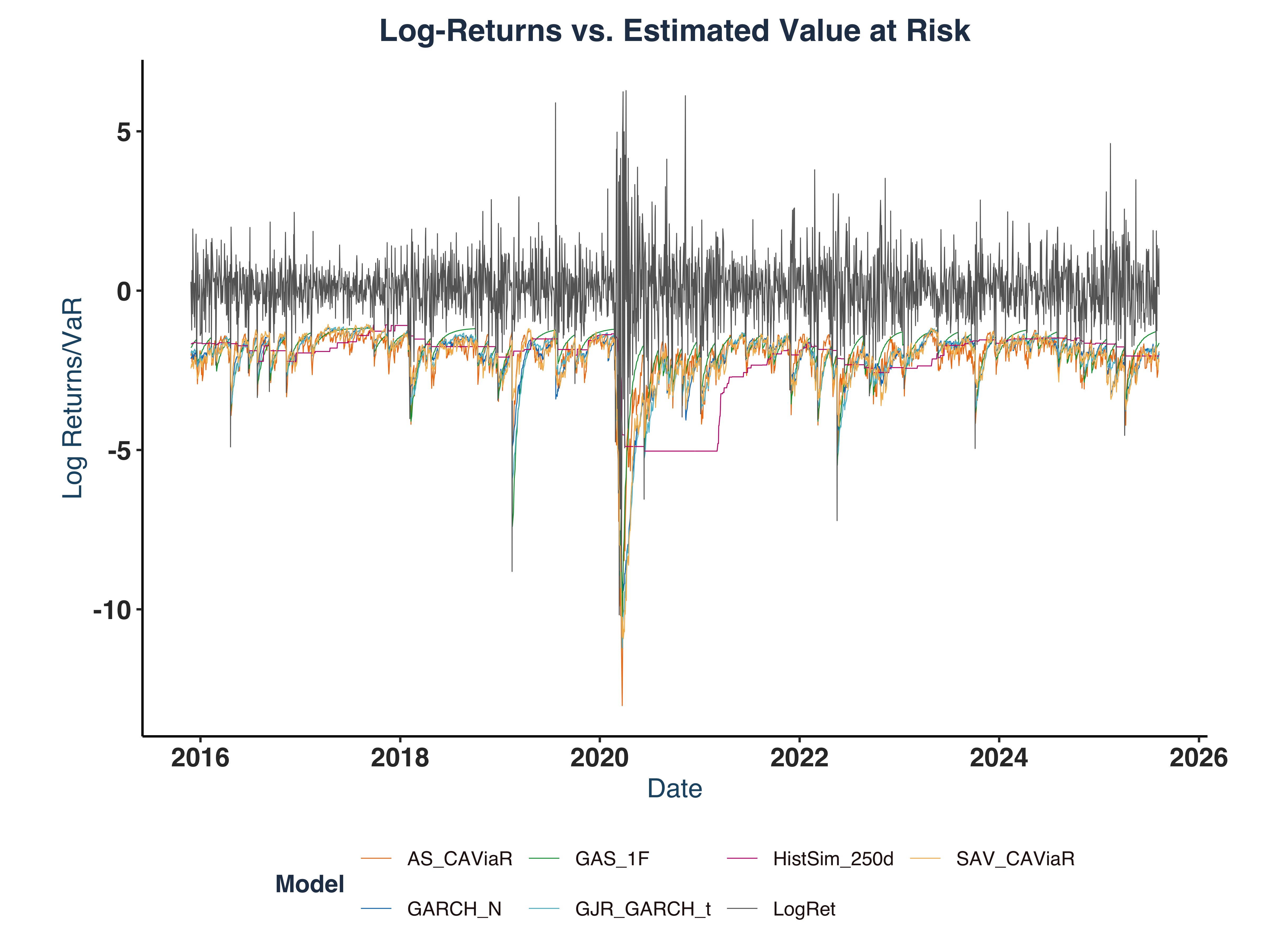
labs(
title = "Log-Returns vs. Estimated Value at Risk",
x = "Date",
y = "Log Returns/VaR",
color = "Model"
)
# Save plot
ggsave(paste0(c("Plots/KO_VaR_plt.pdf")), plot = KO_VaR_plt, width=8, height=6)
# Print
# I recommend the library `plotly` for interactive graph
# ggplotly(KO_VaR_plt, colors = mdl_colors)
KO_VaR_plt
|
ii. Plot ES#
 1
 2
 3
 4
 5
 6
 7
 8
 9
10
11
12
13
14
15
16
17
18
19
20
21
22
23
24
25
26
27
28
29
30
31
32
33
|
## Reshape plot data (wide to long) ----
# Extract ES columns & reshape
es_long_dt <- reshape(KO_qe_plt_dt[,c("date", "ret", paste0("e_", all_mdl_ls))],
                      direction = "long",
                      idvar = "date",
                      varying = c("ret", paste0("e_", all_mdl_ls)), v.names = "value",
                      timevar = "model", times =  c("LogRet", all_mdl_names)
                      )
# Drop row indices
rownames(es_long_dt) <- NULL

KO_ES_plt <- es_long_dt |>
  ggplot(aes(x = date, y = value, color = model)) +
  geom_line(linewidth = 0.2)+
  scale_color_manual(values = mdl_colors)+
  theme(panel.grid.major = element_blank(),
        panel.grid.minor = element_blank(),
        panel.border = element_blank(),
        panel.background = element_blank(),
        legend.position = "bottom"
        ) +
  global_fonts+
  labs(
    title = "Log-Returns vs. Estimated Expected Shortfall",
    x = "Date",
    y = "Log Returns/VaR",
    color = "Model"
  )
# Save plot
ggsave(paste0(c("Plots/KO_ES_plt.pdf")), plot = KO_ES_plt, width=8, height=6)
# Print
# ggplotly(KO_ES_plt) # I recommend the library `plotly` for interactive graph, however it won't compile for pdf export
KO_ES_plt
|
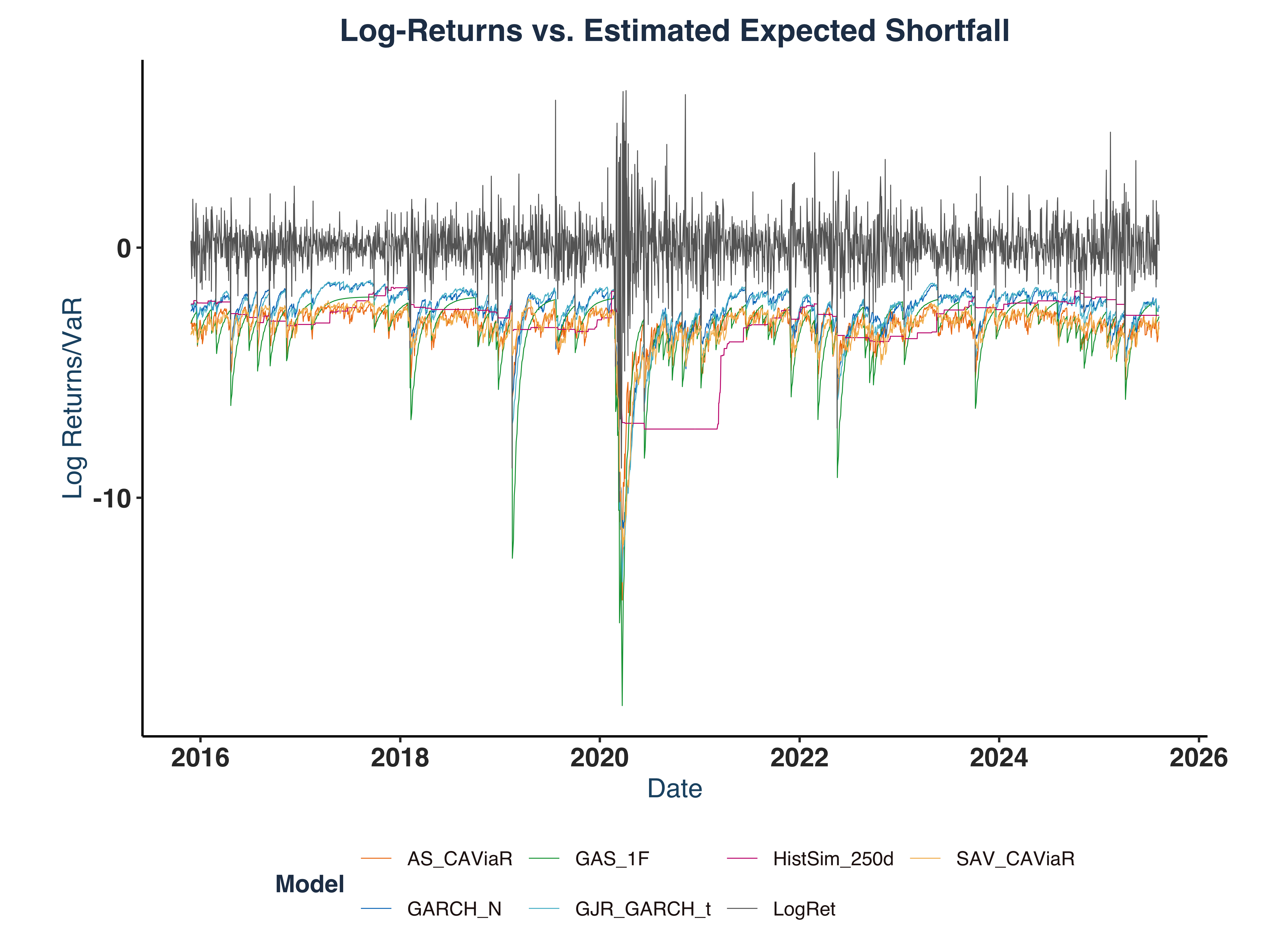
iii. Model Graphical Evaluation#
Plot Main Features:
- A major volatility spike around COVID-19 pandemic, associated with a massive drop by approximately -10%.
- In both VaR and ES plot, all models successfully capture major market volatility.
- GAS-type models seem to be the most responsive model that quickly reflects the market turmoil with sensitive responses, e.g. it predicted a -15.0% drop on 2020-03-13 in response to the -10.2% decline in Log-return on 2020-03-12.
Detailed Models Evaluation:
- GAS-1F: the most responsive model with largest adjustment during volatile periods. It also shows a smooth adaptation post-crisis.
- AS-CAViaR: the second most responsive model most of the time, associated with sharp responses; however, it is sometimes hypersensitive. For example, it estimated a -14.8% decrease in VaR on 2020-03-23 while the realized decline was only -2.0%.
- SAV-CAViaR: a balanced model which is neither too reactive nor too static.
- GARCH-N: a stable, consistent model displaying less noise during calm periods. It also exhibits smoother trajectories than CAViaR-type models.
- GJR-GARCH-t: same as GARCH-N but shows less discontinuity (better smoothness).
- HistSim-250d: an unresponsive model showing slow responses to crises. Poor performance in both volatile & quiet periods.
Which model to choose in which period?
- In volatile periods, GAS-1F shows exceptional responsiveness, which helps capture the tail risks effectively, reduce react time, and mitigate foreseeable losses.
- In calmer periods, GARCH-type models are suitable candidate for stable estimates, which lower possibly false signals and reduce unnecessary trading costs.
e. Compute the Hit-ratio for the conditional quantile models.#
i. Hit Ratio Computation#
 1
 2
 3
 4
 5
 6
 7
 8
 9
10
11
12
13
14
15
16
|
# Extract HITS variables
KO_hit_dt <- select(KO_qe_dt, paste0("hit_",all_mdl_ls))

# Calculate hit ratios
n_est <- nrow(KO_qe_dt)
KO_hit_ratio <- KO_hit_dt %>%
  summarise_all(sum) %>%          # column-wise sum
  mutate_all(\(x) x / n_est) %>%  # anonymous function syntax since R 4.1+
  `colnames<-`(all_mdl_names) %>% # assign column names
  pivot_longer(
      cols = everything(),
      names_to = "Model",
      values_to = "Hit_Ratio"
  )

print(KO_hit_ratio)
|
1
2
3
4
5
6
7
8
9
|
## # A tibble: 6 × 2
##   Model        Hit_Ratio
##   <chr>            <dbl>
## 1 HistSim_250d    0.0304
## 2 GARCH_N         0.0254
## 3 GJR_GARCH_t     0.0242
## 4 AS_CAViaR       0.0246
## 5 SAV_CAViaR      0.0242
## 6 GAS_1F          0.0320
|
ii. Conclusion#
Based on hit ration calculation, I would prefer GJR-GARCH-t model because of its lowest hit ratio.
Exercise 2 - Simulation Exercises#
a. Time Series Examination#
Given five processes:
\(Y_t = Y_{t-1} + \varepsilon_t\): Non-stationary random walk, used as a reference for forecasting, acting as the “best” prediction we can make.\(Y_t = \varepsilon_t\): Stationary White Noise, which is the “best” forecast error we can (hopefully) get \(\varepsilon_t = Y_t - \hat{Y_t}\).\(Y_t = 0.8 + 0.8Y_{t-1} + \varepsilon_t\): Stationary AR(1) process, which can be a candidate model for financial series modelling, a state-space representation of a ARMA(p,q) process, or a case of unit root testing.\(Y_t = \sigma_t\varepsilon_t, \quad \sigma_t^2 = 0.04 + 0.05Y_{t-1}^2 + 0.90\sigma_t^2\): \(Y_t\) itself is not stationary, but the conditional volatility \(\sigma_t\) is. This GARCH(1,1) model captures time-varying risk in financial returns.\(q_t = \sigma_tz_{0.05} \quad \text{and} \quad e_t = \sigma_t\xi_{0.05}\): Stationary 5% VaR & ES, which capture the extreme (negative) tail risk.
b. Process Simulation#
i. Simulate Processes & Plot#
Simulate five processess:
 1
 2
 3
 4
 5
 6
 7
 8
 9
10
11
12
|
set.seed(1340)
ts_rw <- ARMA.sim(1000, 1,0,0)
ts_wn <- ARMA.sim(1000, 0,0,0)
ts_ar1 <- ARMA.sim(1000, 0.8,0,0.8)
ts_garch1 <- GARCH.sim(1000, 0.04, 0.05, 0.9)
ts_eq <- VaR.ES.sim(1000, 0.05, 0.04, 0.05, 0.9)

# Create plot data
ts_plot_dt <- data.frame(time = 1:1000, ts_rw = ts_rw, ts_wn = ts_wn,
                         ts_ar1 = ts_ar1, ts_garch1_y = ts_garch1$y,
                         ts_garch1_sig = ts_garch1$sigma.2,
                         ts_var = ts_eq$q_t, ts_es = ts_eq$e_t)
|
And plot them:
 1
 2
 3
 4
 5
 6
 7
 8
 9
10
11
12
13
14
15
16
17
18
19
20
21
22
23
24
25
26
27
28
29
30
31
32
33
34
35
36
37
38
39
40
|
ts_basic_plt <- ggplot(ts_plot_dt, aes(x=time)) +
  geom_line(aes(y=ts_rw*0.05, colour = "Random Walk"),size=0.5) + # Put to secondary y-axis
  geom_line(aes(y=ts_wn, colour = "White Noise"),size=0.3) +
  geom_line(aes(y=ts_ar1, colour = "AR(1)"),size=0.3) +
  scale_y_continuous(
    name = "White Noise / AR(1)",
    sec.axis = sec_axis(trans = ~ . / 0.05,name = "Random Walk")
  ) +
  theme(panel.grid.major = element_blank(),
        panel.grid.minor = element_blank(),
        panel.border = element_blank(),
        panel.background = element_blank()) +
  global_fonts+
  labs(title = "Basic Time Series Simulation",x = NULL,y = NULL) +
  scale_color_manual(name = "Time Series",
                     values = c("Random Walk" = "#1F6E9CFF",
                                "White Noise" = "#FE9B00FF",
                                "AR(1)"       = "#D8443CFF"))
ts_garch_plt <- ggplot(ts_plot_dt, aes(x=time)) +
  geom_line(aes(y=ts_garch1_y, colour = "GARCH(1,1)"),size=0.3) +
  geom_line(aes(y=ts_garch1_sig, colour = "Cond. Volatility"),size=0.3) +
  geom_line(aes(y=ts_var, colour = "VaR"),size=0.3) +
  geom_line(aes(y=ts_es, colour = "ES"),size=0.3) +
  theme(panel.grid.major = element_blank(),
        panel.grid.minor = element_blank(),
        panel.border = element_blank(),
        panel.background = element_blank()) +
  global_fonts+
  labs(title = "Volatility-based Time Series Simulation",x = NULL,y = NULL) +
  scale_color_manual(name = "Time Series",
                     values = c("GARCH(1,1)" = "#E6A2A6FF",
                                "Cond. Volatility" = "#9B3441FF",
                                "VaR" = "#2B9B81FF",
                                "ES" = "#92C051FF"))

sim_ts_plt <- ggarrange(ts_basic_plt, ts_garch_plt, nrow = 2, widths = 8, heights = 6)

# Save plot
ggsave(paste0(c("Plots/Simulated_Time_Series_plt.pdf")), plot = sim_ts_plt, width=8, height=6)
sim_ts_plt
|
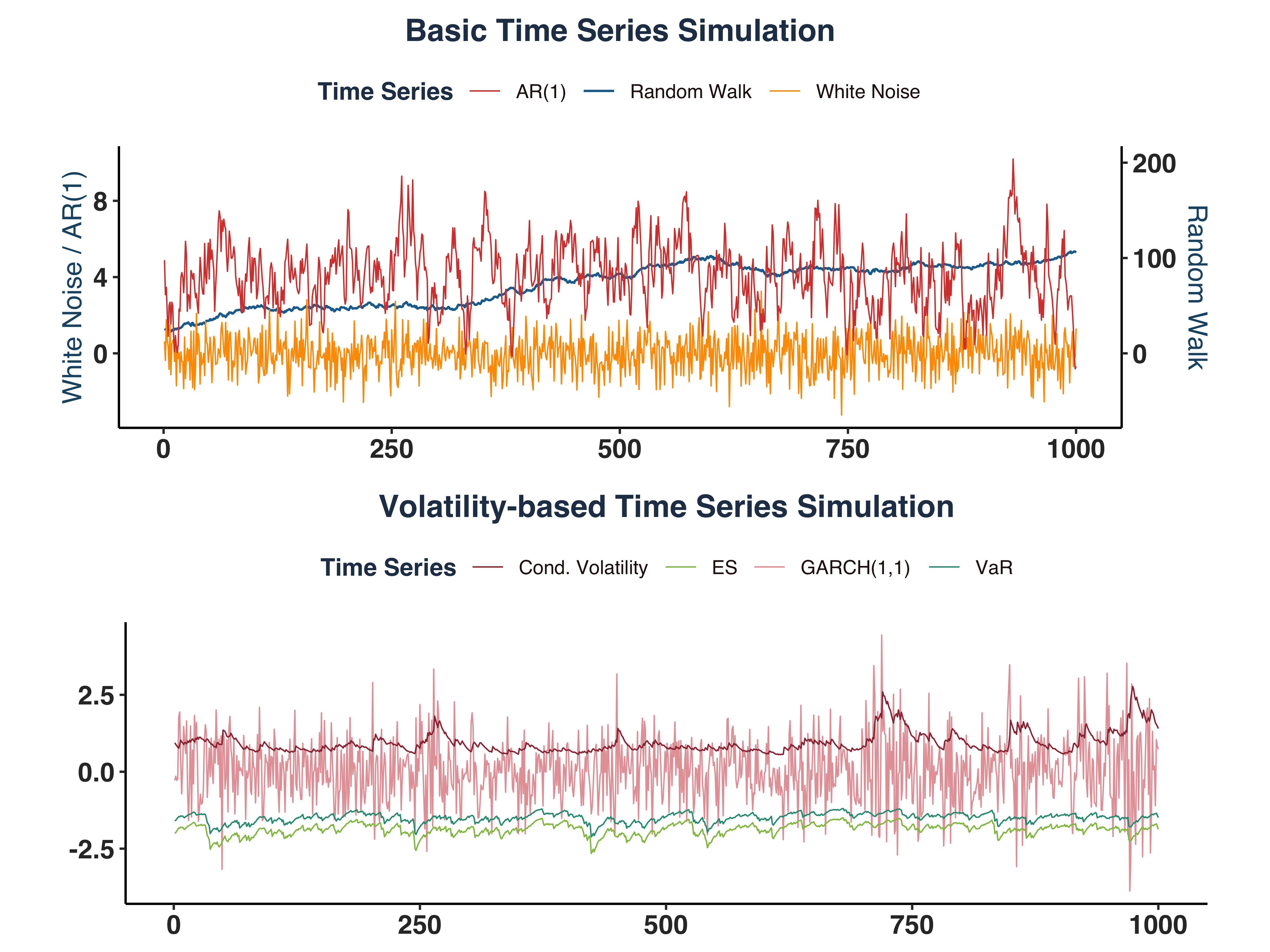
ii. Time Series Behaviour#
- Random Walk series shows a clear upward trend over time.
- Both White Noise (WN) & AR(1) series exhibit mean-reverting properties, where WN stations around 0 and AR(1) series’s mean is 4.
- Conditional Variance series is stationary around 0.8.
- VaR series varies around
\(q_t ={\sigma}_t*z_{0.05}\approx 0.8944*-1.6449=\) -1.4712018
- ES series fluctuates around
\(e_t ={\sigma}_t*\xi_{0.05}\approx 0.8944*-2.0627=\) -1.8449464.
c. Explain Almost Surely (a.s.) Convergence#
-
Intuitively, we can find a bound $\varepsilon > 0 $ that at some point \(n\), the sequence falls under this bound and will never leave it.
-
Formally, a random sequence of sample averages \(\{\bar{Y}_n\}\) converges almost surely if for all \(\omega\in \Omega\) and any \(\varepsilon > 0 \quad \exists \bar{n}(\varepsilon, \omega) \in \mathbb{N}\) such that:
$$
|\bar{Y}_n - \mu| < \varepsilon \quad \forall, n \geq \bar{n}(\varepsilon, \omega)
$$
-
In this context, converging refers to a realization \(\omega\) reverting to its mean \(\mu\).
-
The term \(\bar{n}(\varepsilon, \omega)\) is known as “Convergence Threshold”.
-
Illustration:
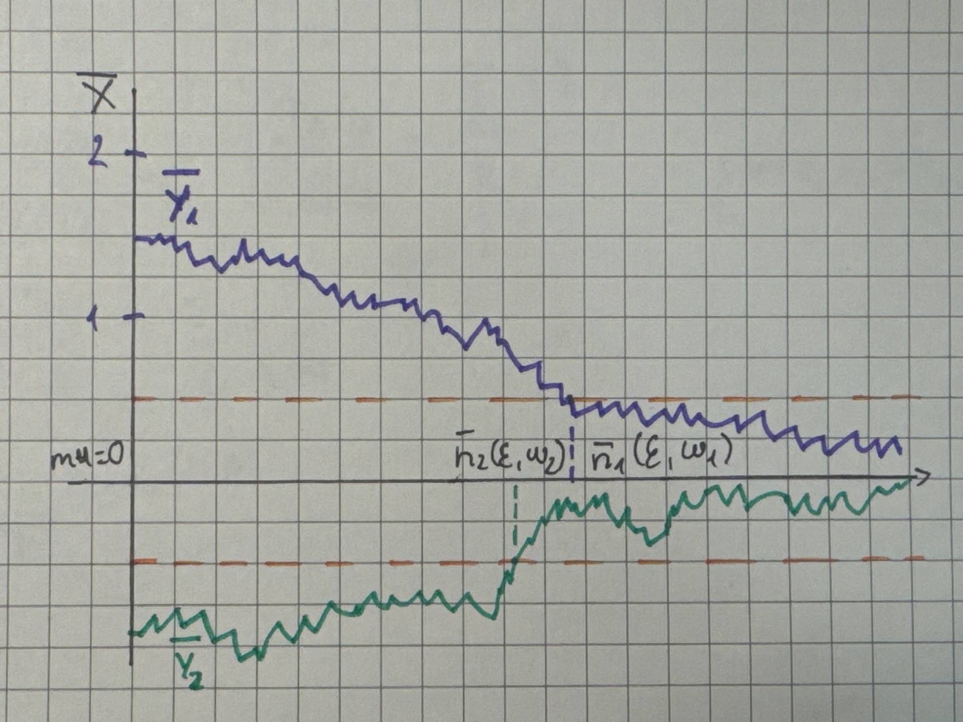 {width=60%}
Note: \(\bar{Y}_1,\bar{Y}_2\) denote different realizations of a time series
d. Explain Convergence in Probability#
- Intuitively, if we assess the probability that the series falls under the defined bound and never go out:
\(\lim_{n\to \infty} p_n = \lim_{n\to \infty} P\left( |\bar X_n - \mu| > \varepsilon\right)=0\)
- Formally, a sequence of random variables
\(\{X_n\}\) is said to converge in probability to a random variable \(X\) if for any \(\varepsilon>0\):
$$
\lim_{n\to \infty} P\left( | X_n - X| > \varepsilon\right)=0
$$
- In this context,
\(p_n = p_T\) means the probability of absolute deviation between \(\bar{X}_T\) and the limit/mean \(\mu\) by more than \(\varepsilon\) equals to zero at time \(T\).
- In common sense, the probability of getting an out-of-hand observation collapses to zero as sample size grow.
- Demonstration:
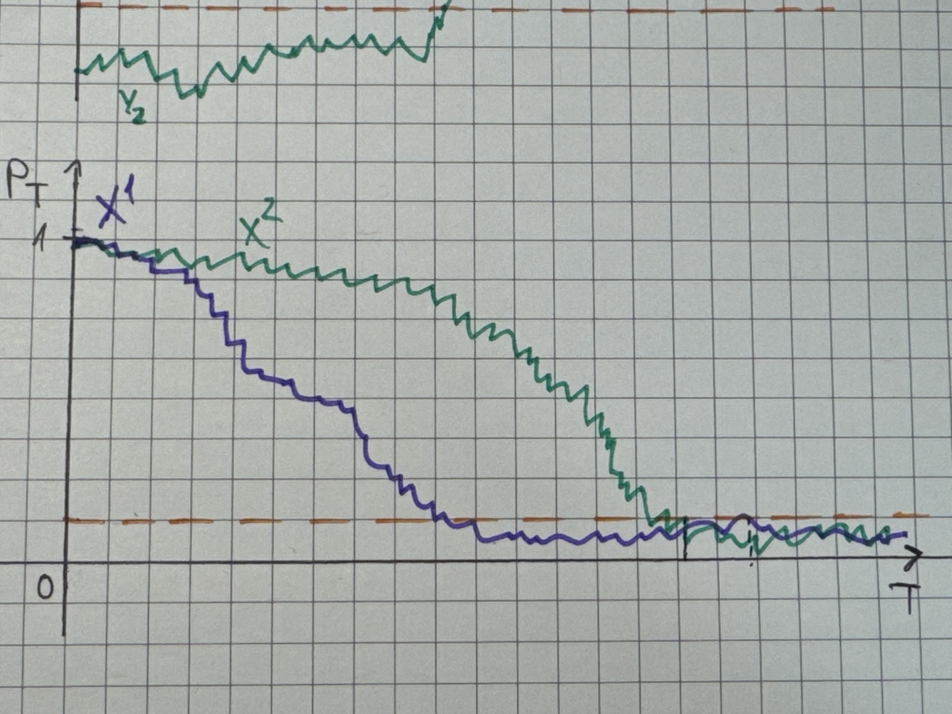 {width=60%}
Note: \(X^1,X^2\) denote different time series
e. Simulation & Convergence#
i. Simulate Stationary Processes#
 1
 2
 3
 4
 5
 6
 7
 8
 9
10
11
12
13
14
15
16
17
18
19
20
21
22
23
24
25
26
27
28
29
|
# Simulate the time series
set.seed(1340)
T_obs <- 10000
sta_ts_wn <- ARMA.sim(T_obs, 0,0,0, ensembles = 4)
sta_ts_ar1 <- ARMA.sim(T_obs, 0.8,0,0.8, ensembles = 4)
sta_ts_garch11 <- GARCH.sim(T_obs, 0.04, 0.05, 0.9, ensembles = 4)
sta_ts_eq <- VaR.ES.sim(T_obs, 0.05, 0.04, 0.05, 0.9, ensembles = 4)

# Compute sequence of averages
mean_wn <- as.data.frame(apply(sta_ts_wn, 2, \(x) cumsum(x)/seq_along(x)))
mean_ar1 <- as.data.frame(apply(sta_ts_ar1, 2, \(x) cumsum(x)/seq_along(x)))
mean_g11 <- as.data.frame(apply(sta_ts_garch11$sigma.2, 2, \(x) cumsum(x)/seq_along(x)))
mean_qt <- as.data.frame(apply(sta_ts_eq$q_t, 2, \(x) cumsum(x)/seq_along(x)))
mean_et <- as.data.frame(apply(sta_ts_eq$e_t, 2, \(x) cumsum(x)/seq_along(x)))

# Compute deviations
eps <- 0.01
abs_dev_wn_dt <- as.data.frame(abs(mean_wn-0))      # mu=0
abs_dev_ar1_dt <- as.data.frame(abs(mean_ar1-4))    # mu=4
abs_dev_g11_dt <- as.data.frame(abs(mean_g11-0.8))  # mu=0.8
mu_var <- sqrt(0.8)*qnorm(0.05, 0, 1)
abs_dev_qt_dt <- as.data.frame(abs(mean_qt-mu_var)) # mu=-1.4712
mu_es <- sqrt(0.8)*(-dnorm(qnorm(0.05, 0, 1), 0, 1) / 0.05)
abs_dev_et_dt <- as.data.frame(abs(mean_et-mu_es))  # mu=-1.8449

# Set names
col_names <- c("Ensemble_1","Ensemble_2","Ensemble_3","Ensemble_4")
list2env(lapply(mget(c("mean_wn", "mean_ar1", "mean_g11","mean_qt", "mean_et")),
                \(x) setNames(x, col_names)), envir = .GlobalEnv)
|
1
|
## <environment: R_GlobalEnv>
|
1
2
3
|
list2env(lapply(mget(c("abs_dev_wn_dt", "abs_dev_ar1_dt", "abs_dev_g11_dt",
                       "abs_dev_qt_dt", "abs_dev_et_dt")),
                \(x) setNames(x, col_names)), envir = .GlobalEnv)
|
1
|
## <environment: R_GlobalEnv>
|
1
2
3
|
# Create plot data
list2env(lapply(mget(c("mean_wn", "mean_ar1", "mean_g11","mean_qt", "mean_et")),
                \(x) cbind(Index = seq_len(T_obs), x)), envir = .GlobalEnv)
|
1
|
## <environment: R_GlobalEnv>
|
1
2
|
# Print out a series to check
tail(mean_ar1, 10)
|
 1
 2
 3
 4
 5
 6
 7
 8
 9
10
11
|
##       Index Ensemble_1 Ensemble_2 Ensemble_3 Ensemble_4
## 9991   9991   4.030821   3.916929   4.005732   3.940538
## 9992   9992   4.031012   3.916674   4.005941   3.940475
## 9993   9993   4.031150   3.916485   4.006032   3.940537
## 9994   9994   4.031361   3.916428   4.006151   3.940445
## 9995   9995   4.031575   3.916271   4.006427   3.940344
## 9996   9996   4.031858   3.916241   4.006735   3.940357
## 9997   9997   4.032243   3.916395   4.007083   3.940438
## 9998   9998   4.032407   3.916415   4.007275   3.940424
## 9999   9999   4.032550   3.916517   4.007449   3.940347
## 10000 10000   4.032733   3.916576   4.007534   3.940287
|
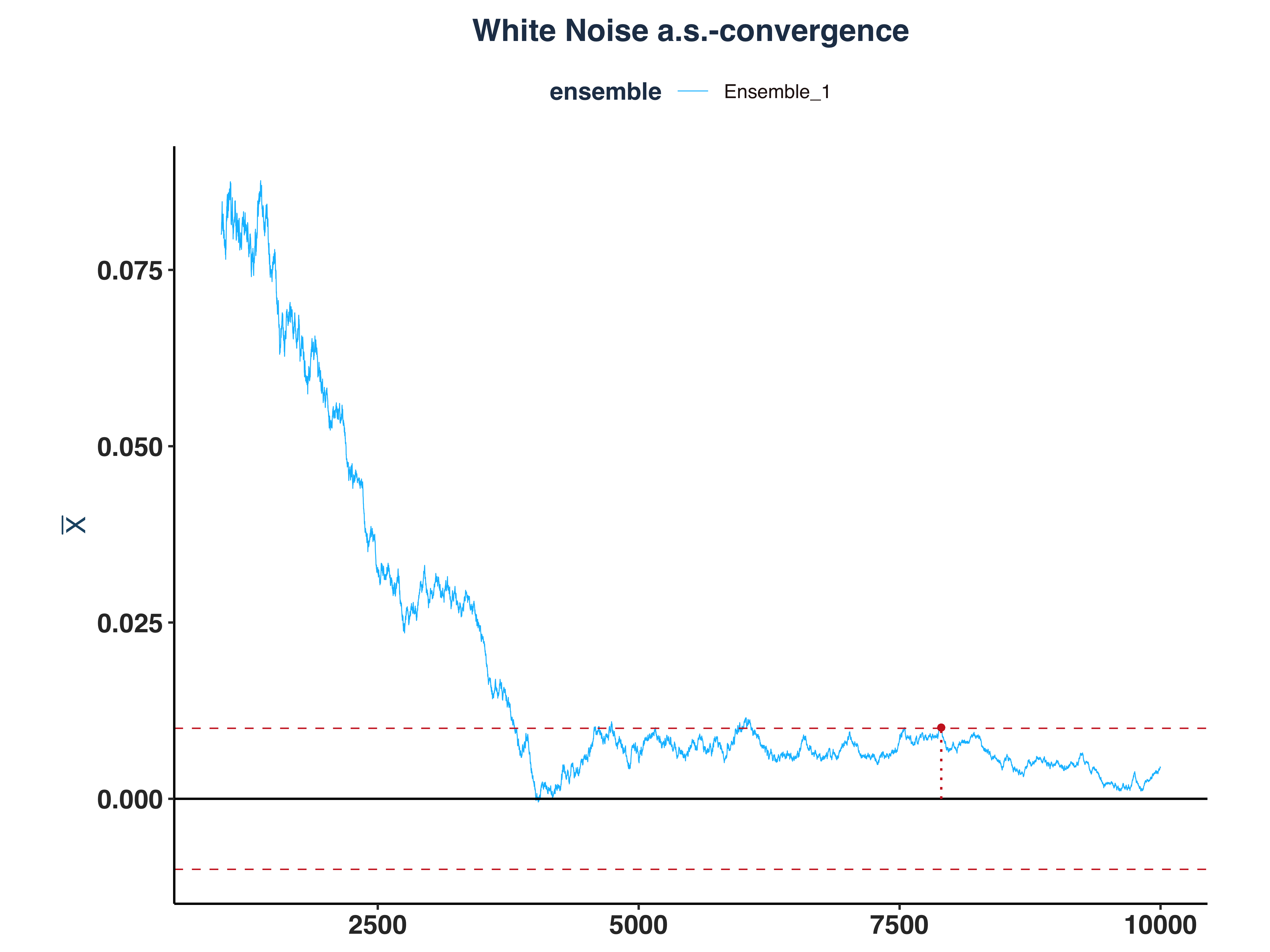
ii. Illustrate a.s.-convergence#
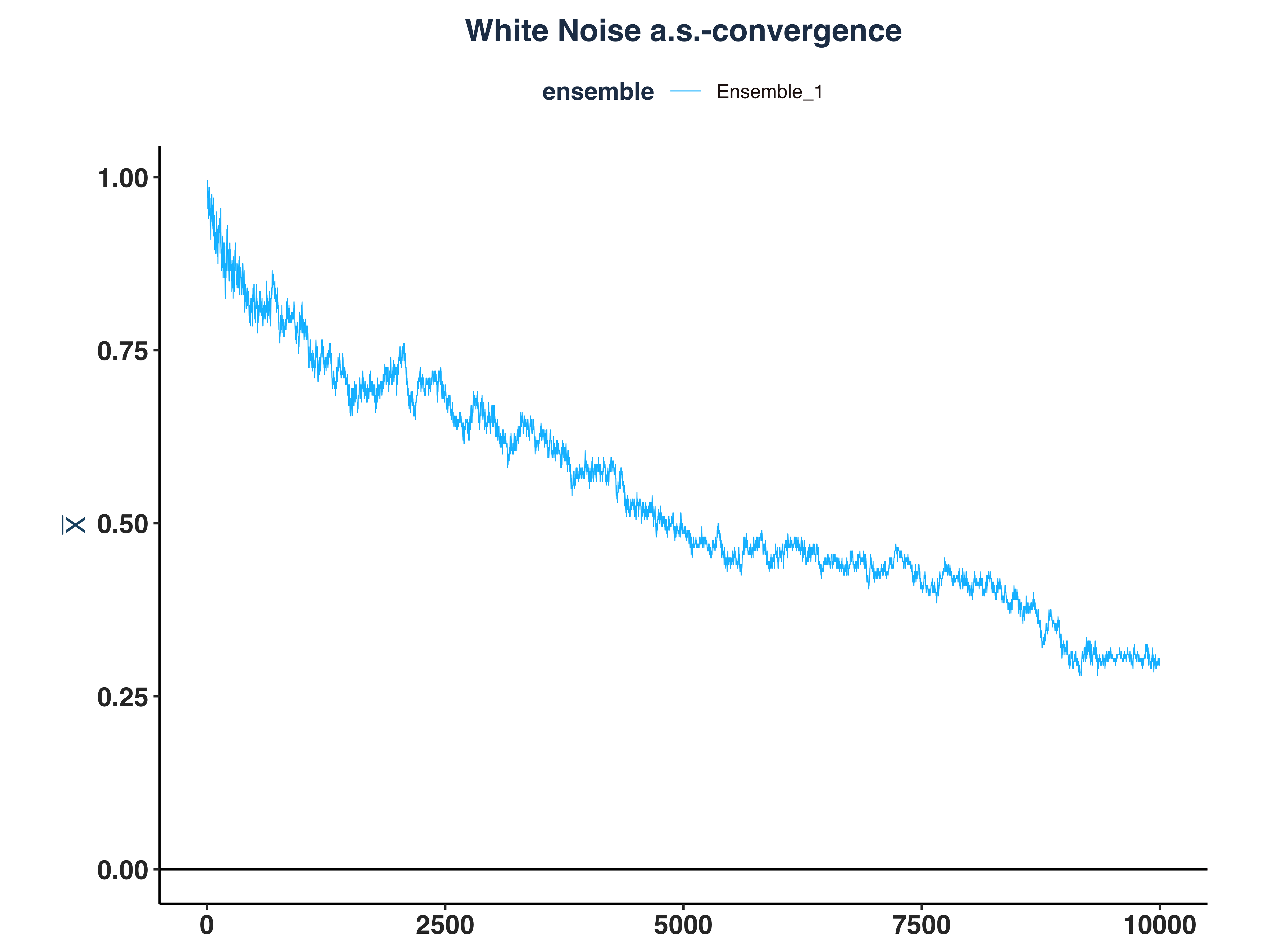
1. White Noise a.s.-convergence
 1
 2
 3
 4
 5
 6
 7
 8
 9
10
11
12
13
|
# Compute \bar{n}(\epsilon, \omega)
n_idx_wn <- apply(abs_dev_wn_dt>eps, 2, \(x) {
  rs <- rev(cumsum(rev(as.numeric(x))))
  idx <- max(which(rs==1))
  `if`(idx == length(x), NULL, idx) # Set to NULL if don't converge
})

# Since the first few hundreds means are so big, I cut them off for better visibility
wn_as_conv_plt <- plot_convergence(mean_wn[1000:10000,], n_idx_wn, "White Noise", "Ensemble_1", eps)

ggsave("Plots/White_Noise_as_convergence.pdf", wn_as_conv_plt,
       width = 8, height = 6, dpi = 300)
wn_as_conv_plt
|
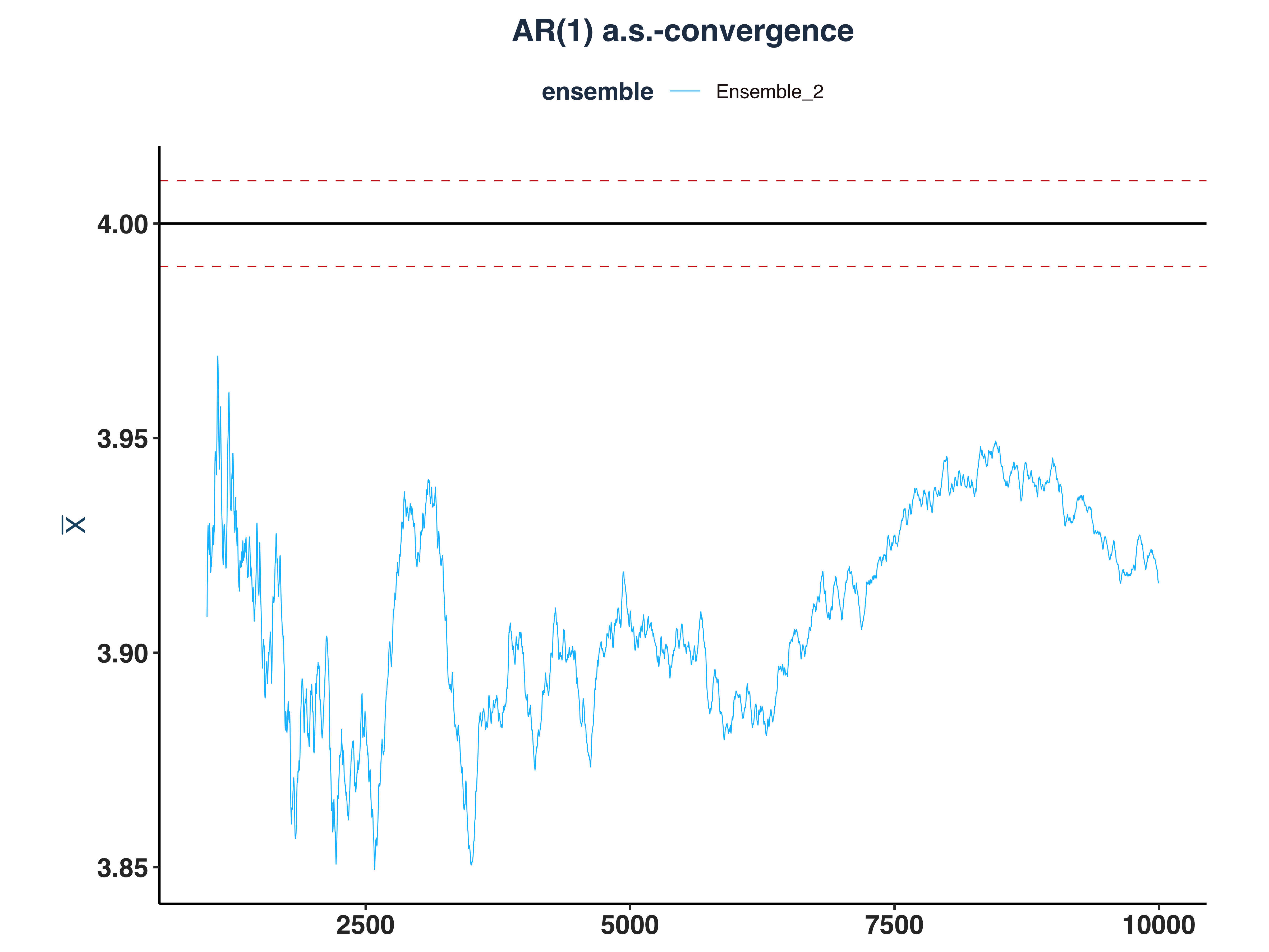
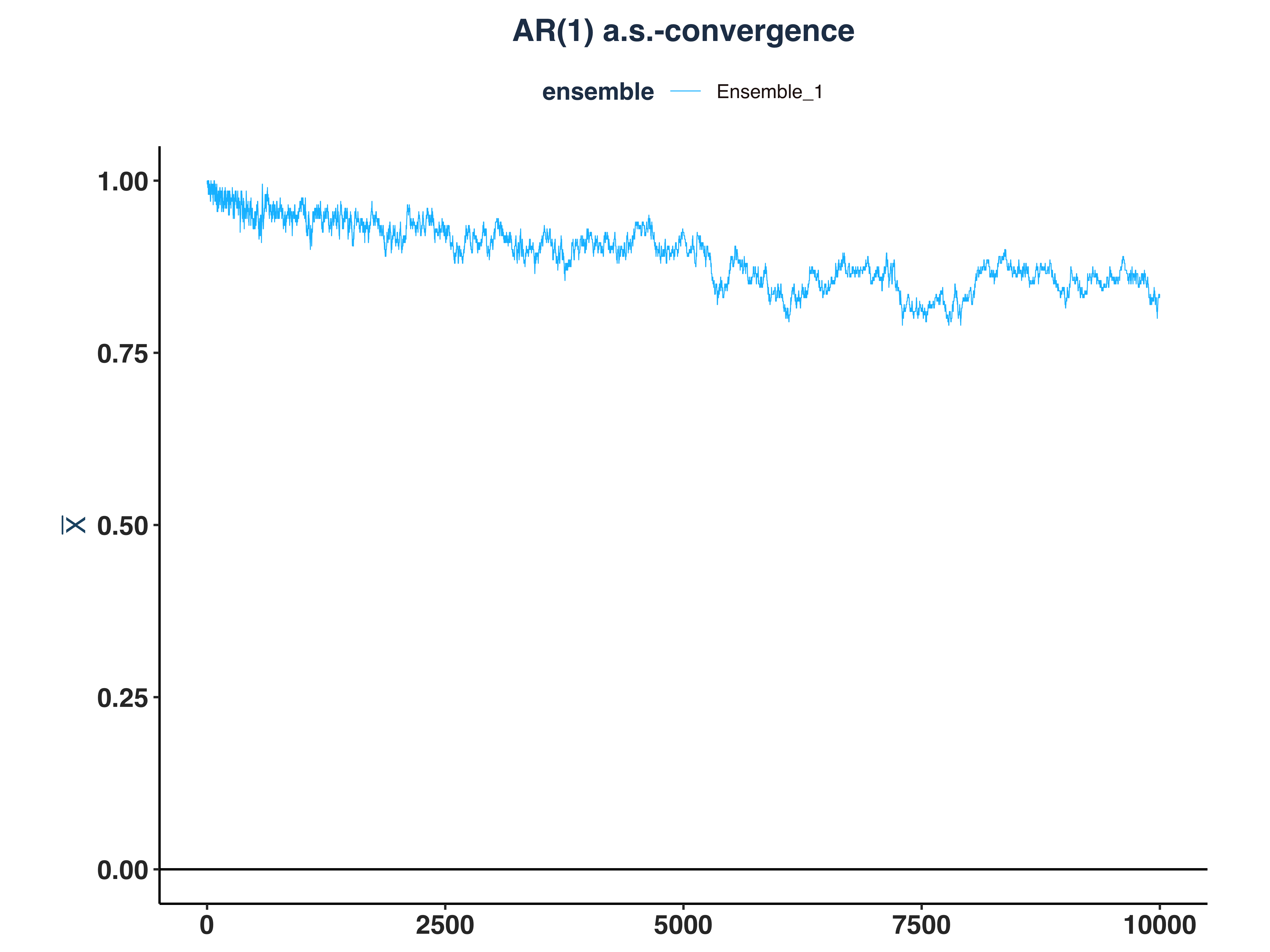
2. AR(1) a.s.-convergence
 1
 2
 3
 4
 5
 6
 7
 8
 9
10
11
12
13
14
|
# Compute \bar{n}(\epsilon, \omega)
n_idx_ar1 <- apply(abs_dev_ar1_dt>eps, 2, \(x) {
  rs <- rev(cumsum(rev(as.numeric(x))))
  idx <- max(which(rs==1))
  `if`(idx == length(x), NULL, idx) # Set to NULL if don't converge
})

# Since the first few hundreds means are so big, I cut them off for better visibility
ar1_as_conv_plt <- plot_convergence(mean_ar1[1000:10000,], n_idx_ar1,
                                    "AR(1)", "Ensemble_2", eps, mu = 4)

ggsave("Plots/AR1_as_convergence.pdf", ar1_as_conv_plt,
       width = 8, height = 6, dpi = 300)
ar1_as_conv_plt
|
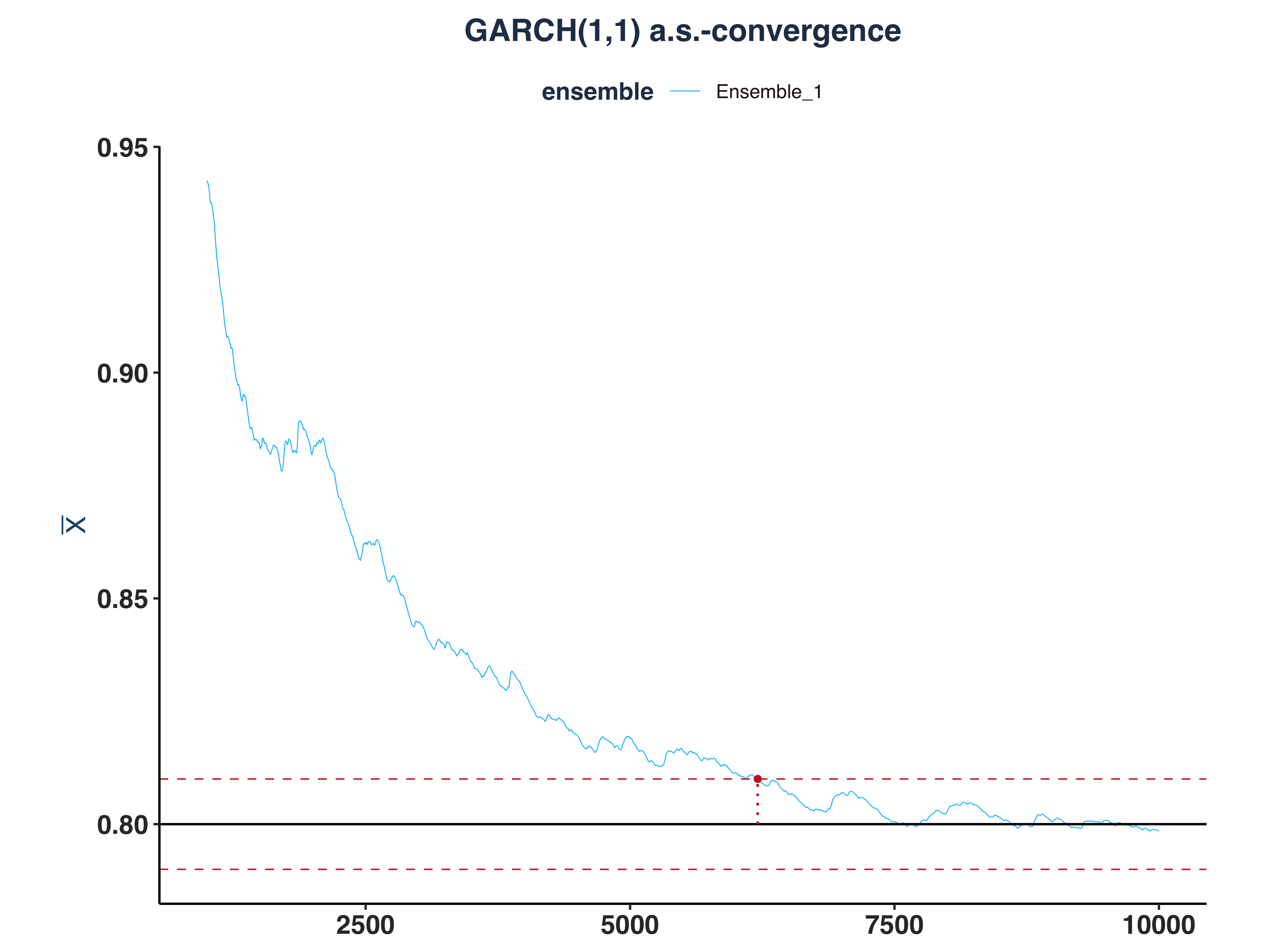
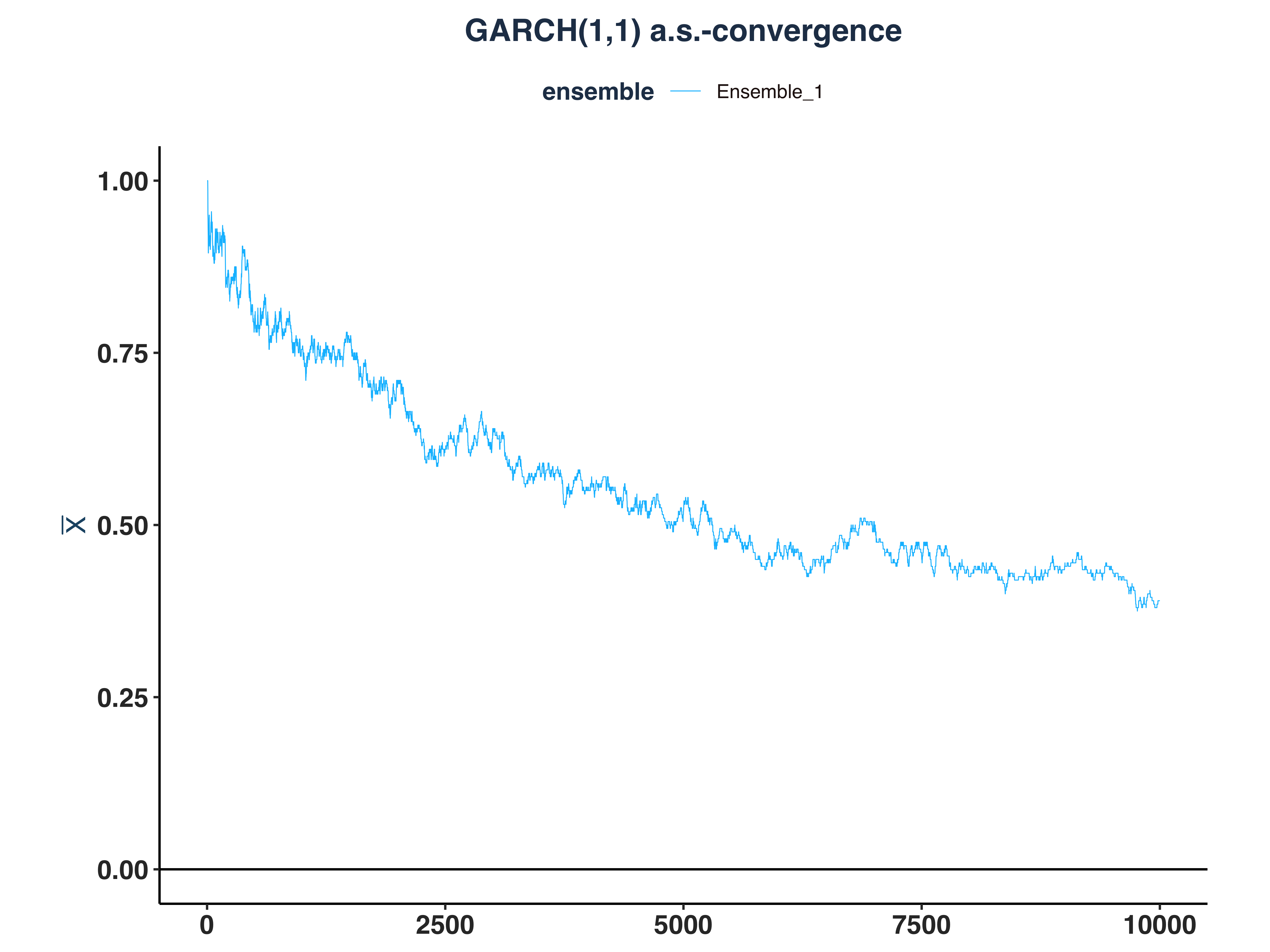
3. GARCH(1,1) a.s.-convergence
 1
 2
 3
 4
 5
 6
 7
 8
 9
10
11
12
13
14
|
# Compute \bar{n}(\epsilon, \omega)
n_idx_g11 <- apply(abs_dev_g11_dt>eps, 2, \(x) {
  rs <- rev(cumsum(rev(as.numeric(x))))
  idx <- max(which(rs==1))
  `if`(idx == length(x), NULL, idx) # Set to NULL if don't converge
})

# Since the first few hundreds means are so big, I cut them off for better visibility
g11_as_conv_plt <- plot_convergence(mean_g11[1000:10000,], n_idx_g11,
                                    "GARCH(1,1)", "Ensemble_1", eps, mu = 0.8)

ggsave("Plots/GARCH11_as_convergence.pdf", g11_as_conv_plt,
       width = 8, height = 6, dpi = 300)
g11_as_conv_plt
|
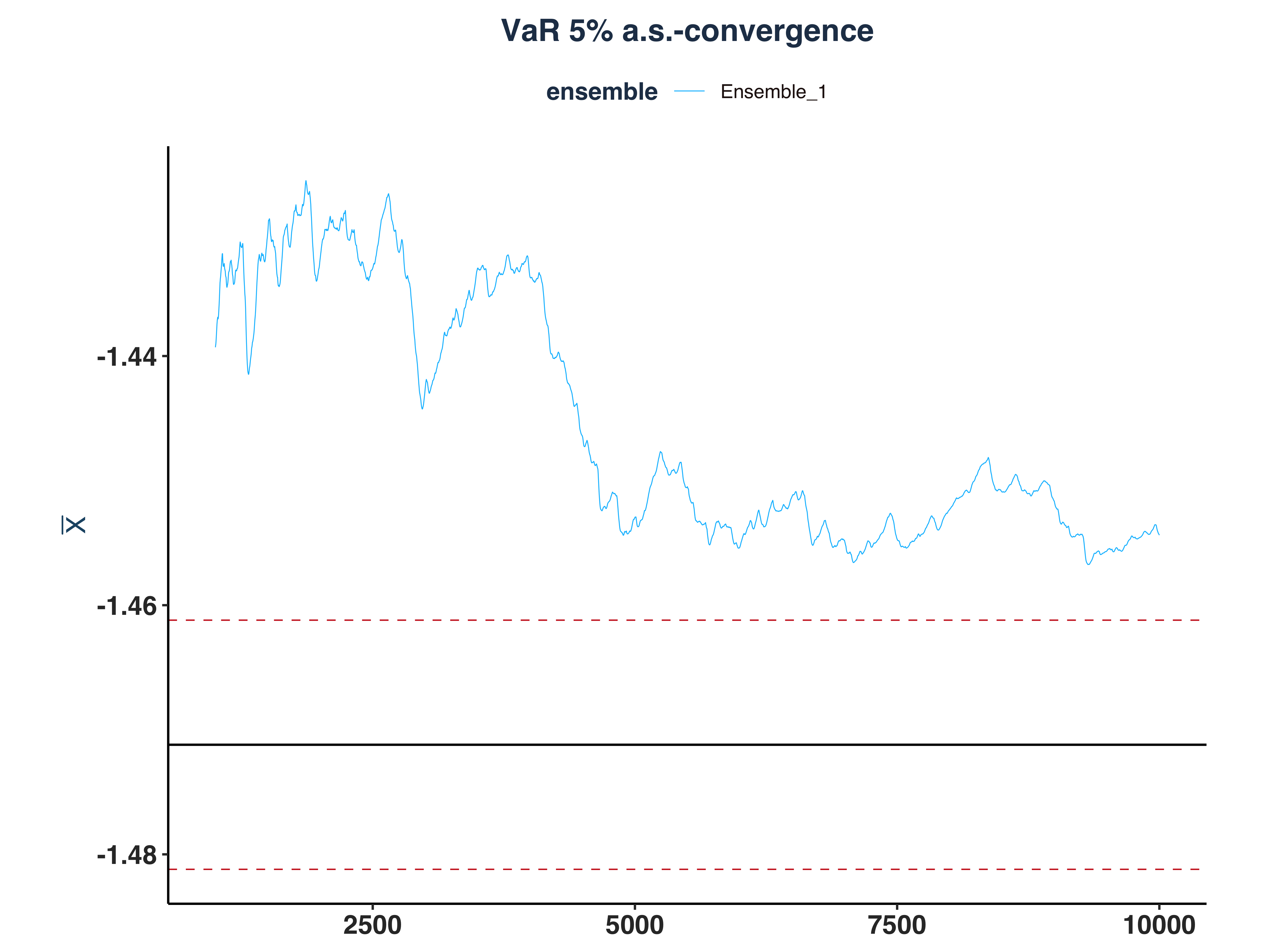
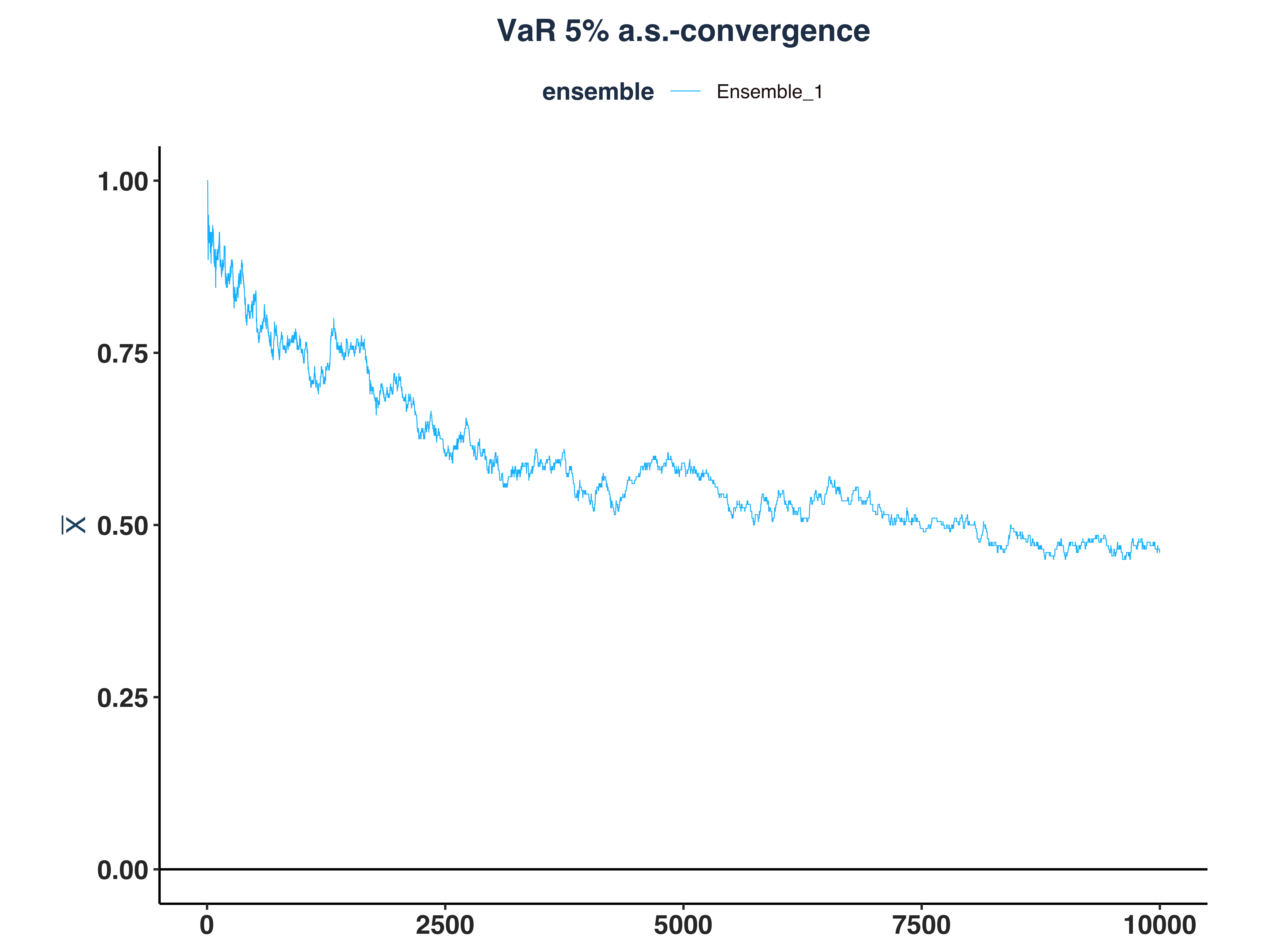
4. VaR 5% a.s.-convergence
 1
 2
 3
 4
 5
 6
 7
 8
 9
10
11
12
13
14
|
# Compute \bar{n}(\epsilon, \omega)
n_idx_var <- apply(abs_dev_qt_dt>eps, 2, \(x) {
  rs <- rev(cumsum(rev(as.numeric(x))))
  idx <- max(which(rs==1))
  `if`(idx == length(x), NULL, idx) # Set to NULL if don't converge
})

# Since the first few hundreds means are so big, I cut them off for better visibility
var_as_conv_plt <- plot_convergence(mean_qt[1000:10000,], n_idx_var,
                                    "VaR 5%", "Ensemble_1", eps, mu = mu_var)

ggsave("Plots/VaR_5pct_as_convergence.pdf", var_as_conv_plt,
       width = 8, height = 6, dpi = 300)
var_as_conv_plt
|
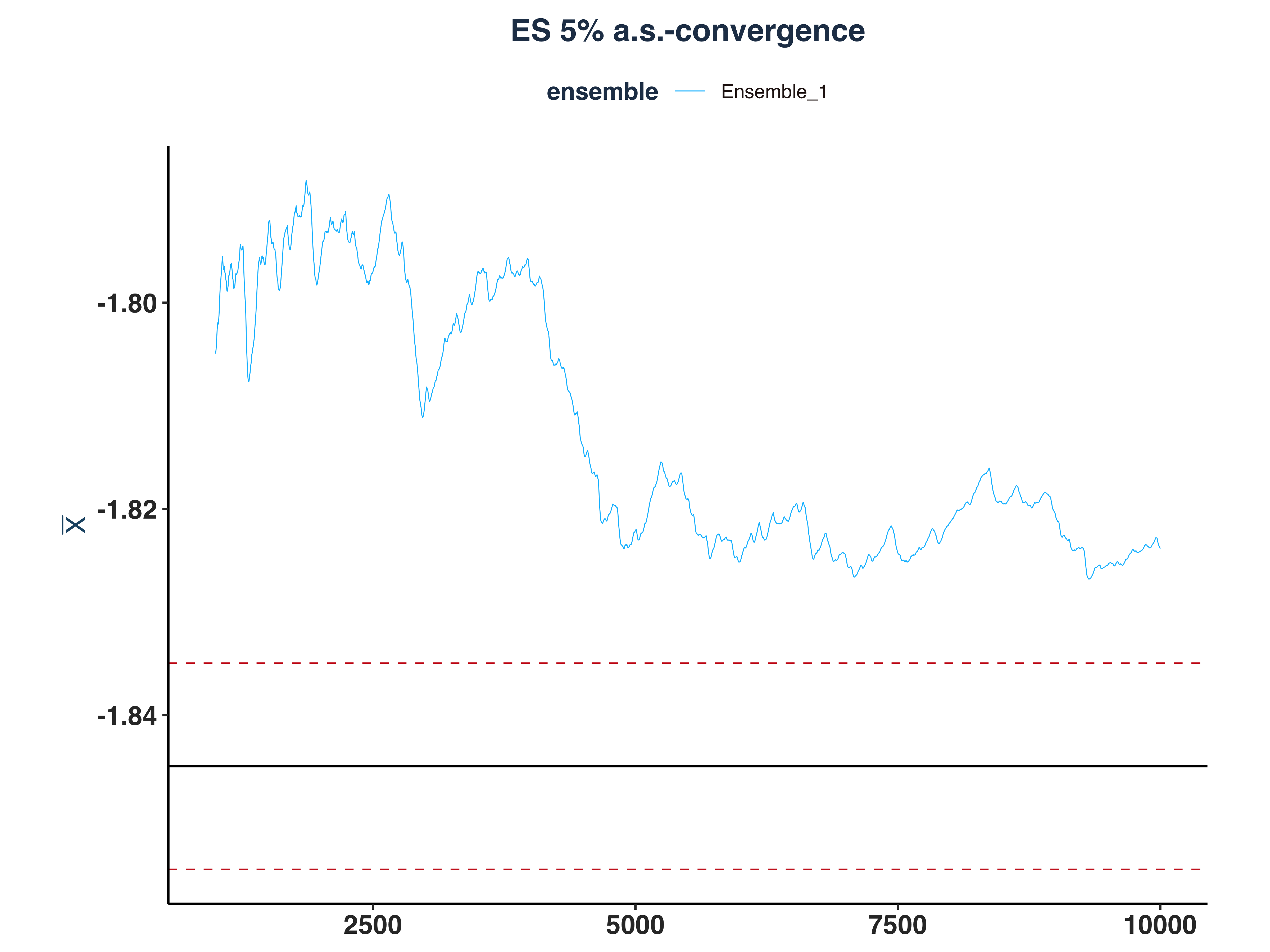
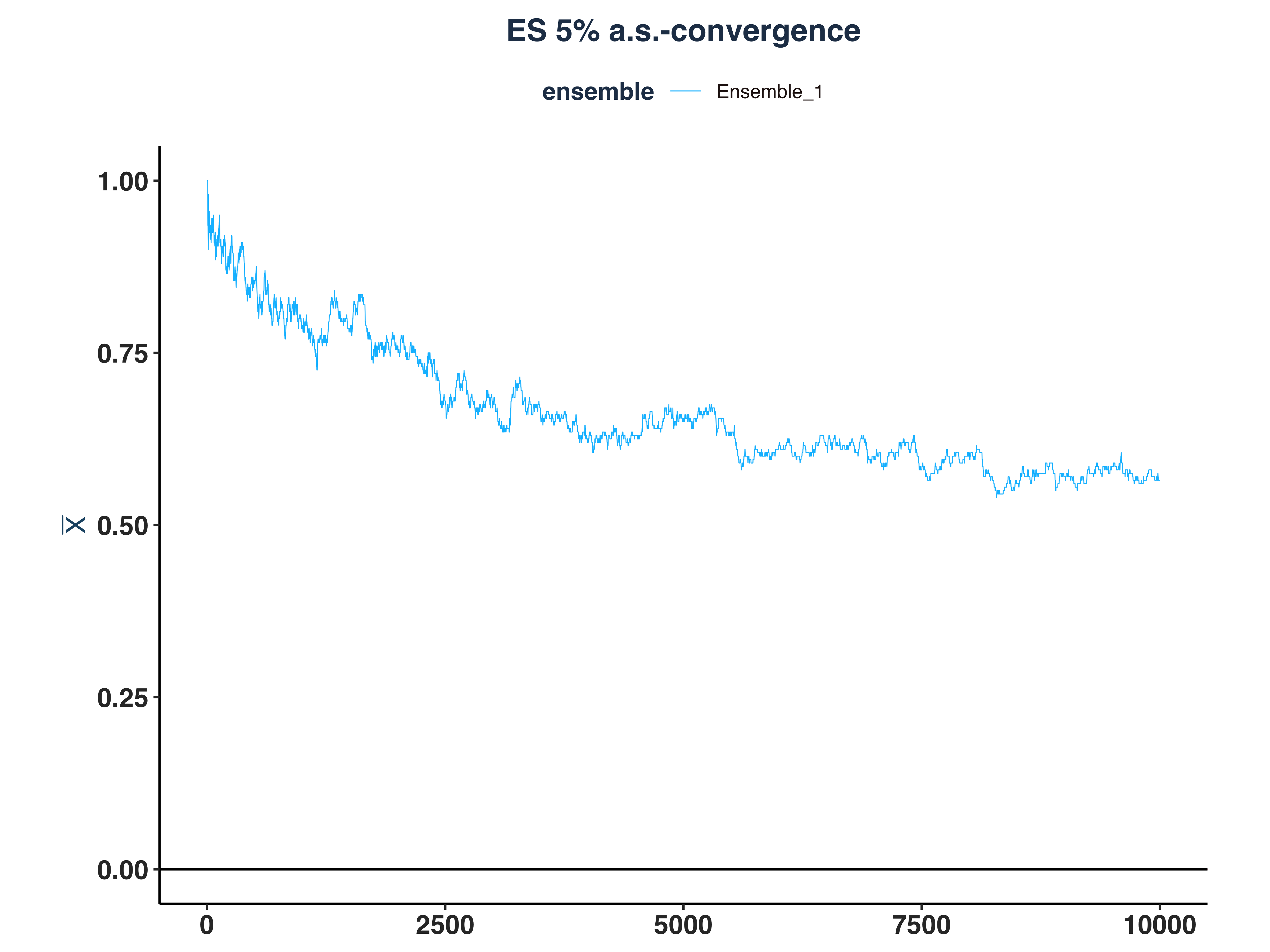
5. ES 5% a.s.-convergence
 1
 2
 3
 4
 5
 6
 7
 8
 9
10
11
12
13
14
|
# Compute \bar{n}(\epsilon, \omega)
n_idx_es <- apply(abs_dev_et_dt>eps, 2, \(x) {
  rs <- rev(cumsum(rev(as.numeric(x))))
  idx <- max(which(rs==1))
  `if`(idx == length(x), NULL, idx) # Set to NULL if don't converge
})

# Since the first few hundreds means are so big, I cut them off for better visibility
es_as_conv_plt <- plot_convergence(mean_et[1000:10000,], n_idx_es,
                                    "ES 5%", "Ensemble_1", eps, mu = mu_es)

ggsave("Plots/ES_5pct_as_convergence.pdf", es_as_conv_plt,
       width = 8, height = 6, dpi = 300)
es_as_conv_plt
|
iii. Repeat for Four Ensembles#
1. White Noise a.s.-convergence
1
2
3
4
5
6
7
|
# Since the first few hundreds means are so big, I cut them off for better visibility
all_wn_as_conv_plt <- plot_convergence(mean_wn[1000:10000,], n_idx_wn,
                                       "White Noise", "all", eps)

ggsave("Plots/All_White_Noise_as_convergence.pdf", all_wn_as_conv_plt,
       width = 8, height = 6, dpi = 300)
all_wn_as_conv_plt
|
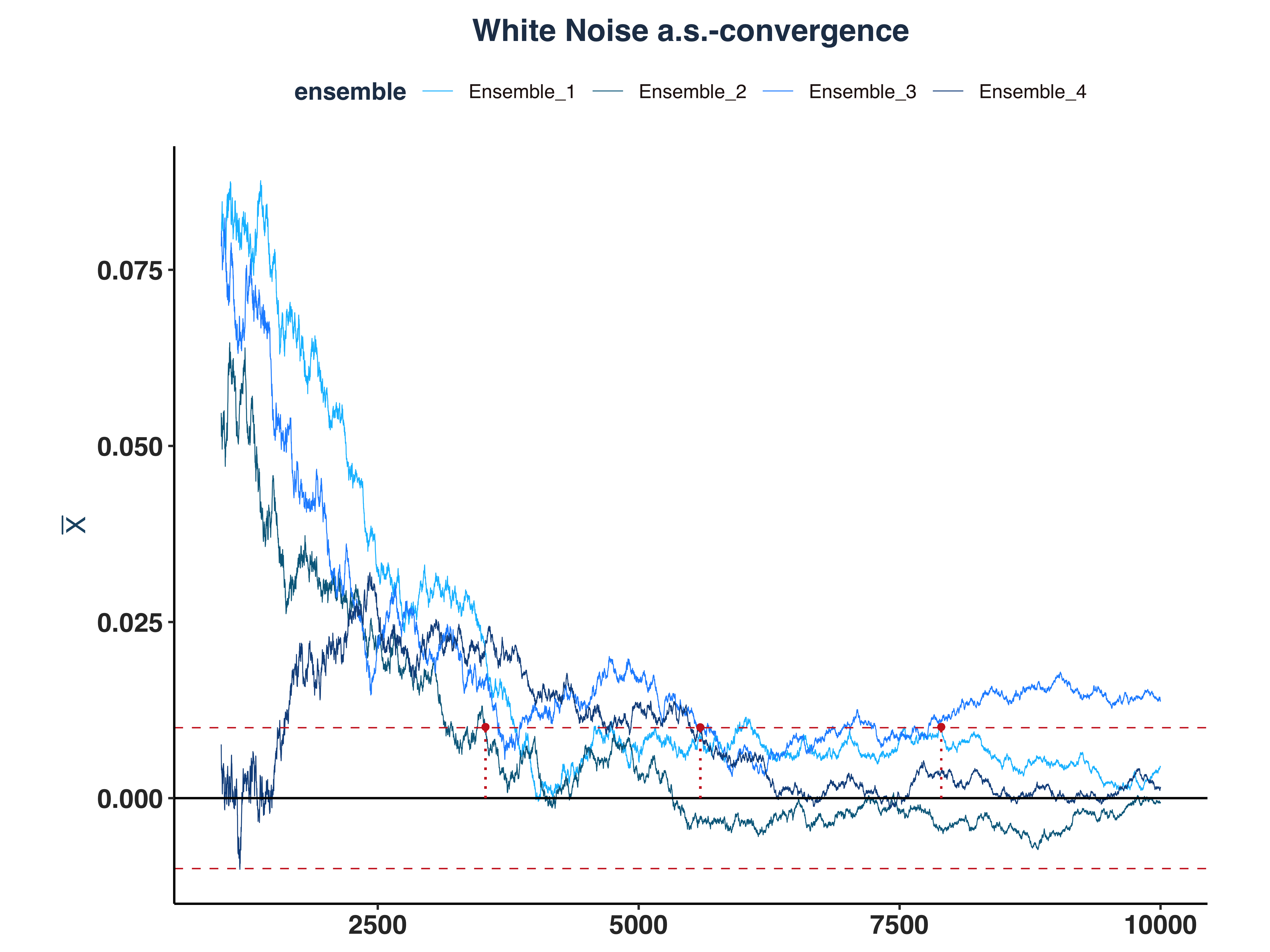
As we can see, only 3 ensembles converged.
2. AR(1) a.s.-convergence
1
2
3
4
5
6
7
|
# Since the first few hundreds means are so big, I cut them off for better visibility
all_ar1_as_conv_plt <- plot_convergence(mean_ar1[1000:10000,], n_idx_ar1,
                                        "AR(1)", "all", eps, mu = 4)

ggsave("Plots/All_AR1_as_convergence.pdf", all_ar1_as_conv_plt,
       width = 8, height = 6, dpi = 300)
all_ar1_as_conv_plt
|
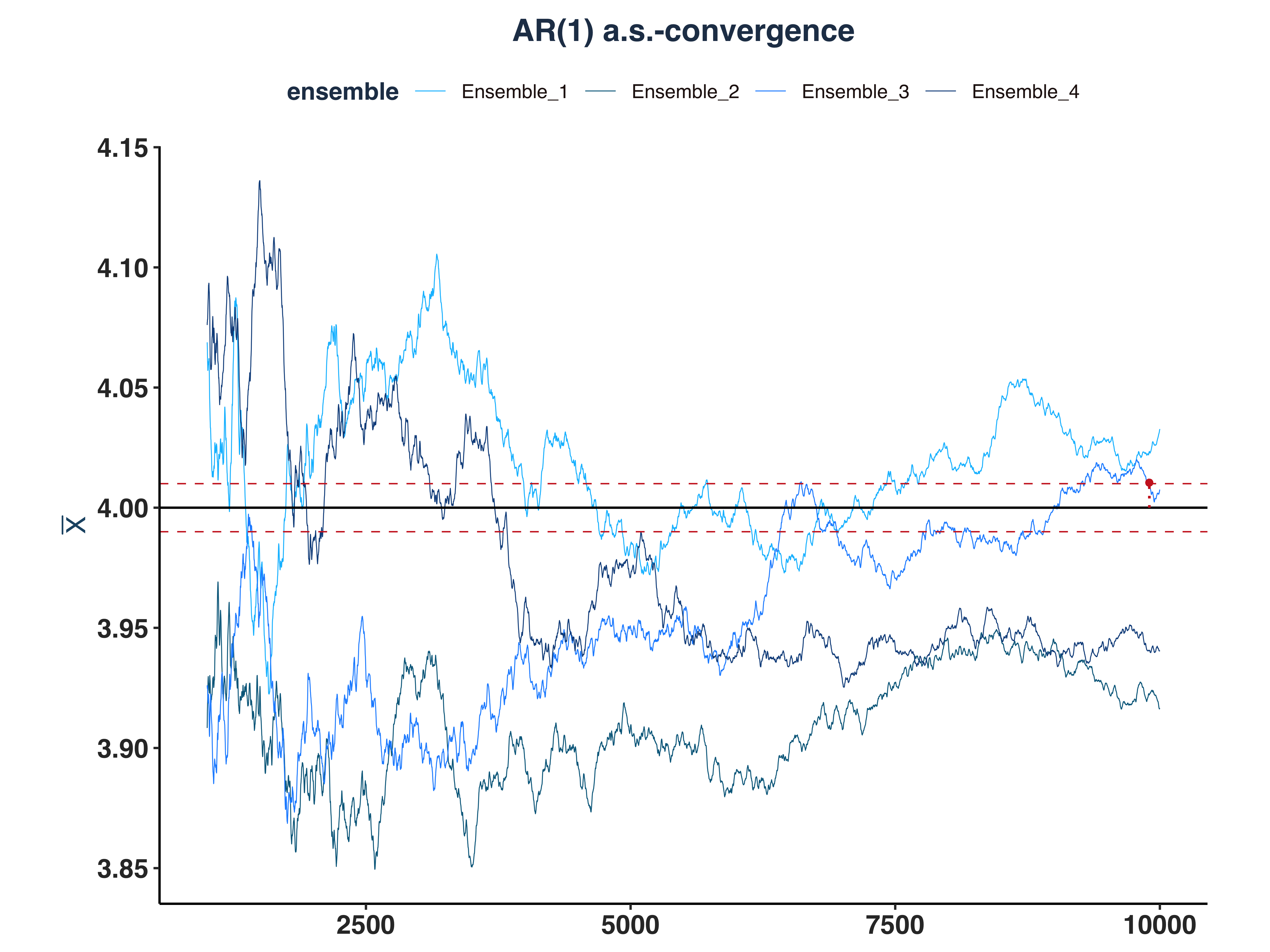
As we can see, only 1 ensemble converged.
3. GARCH(1,1) a.s.-convergence
1
2
3
4
5
6
7
|
# Since the first few hundreds means are so big, I cut them off for better visibility
all_g11_as_conv_plt <- plot_convergence(mean_g11[1000:10000,], n_idx_g11,
                                        "GARCH(1,1)", "all", eps, mu = 0.8)

ggsave("Plots/All_GARCH11_as_convergence.pdf", all_g11_as_conv_plt,
       width = 8, height = 6, dpi = 300)
all_g11_as_conv_plt
|
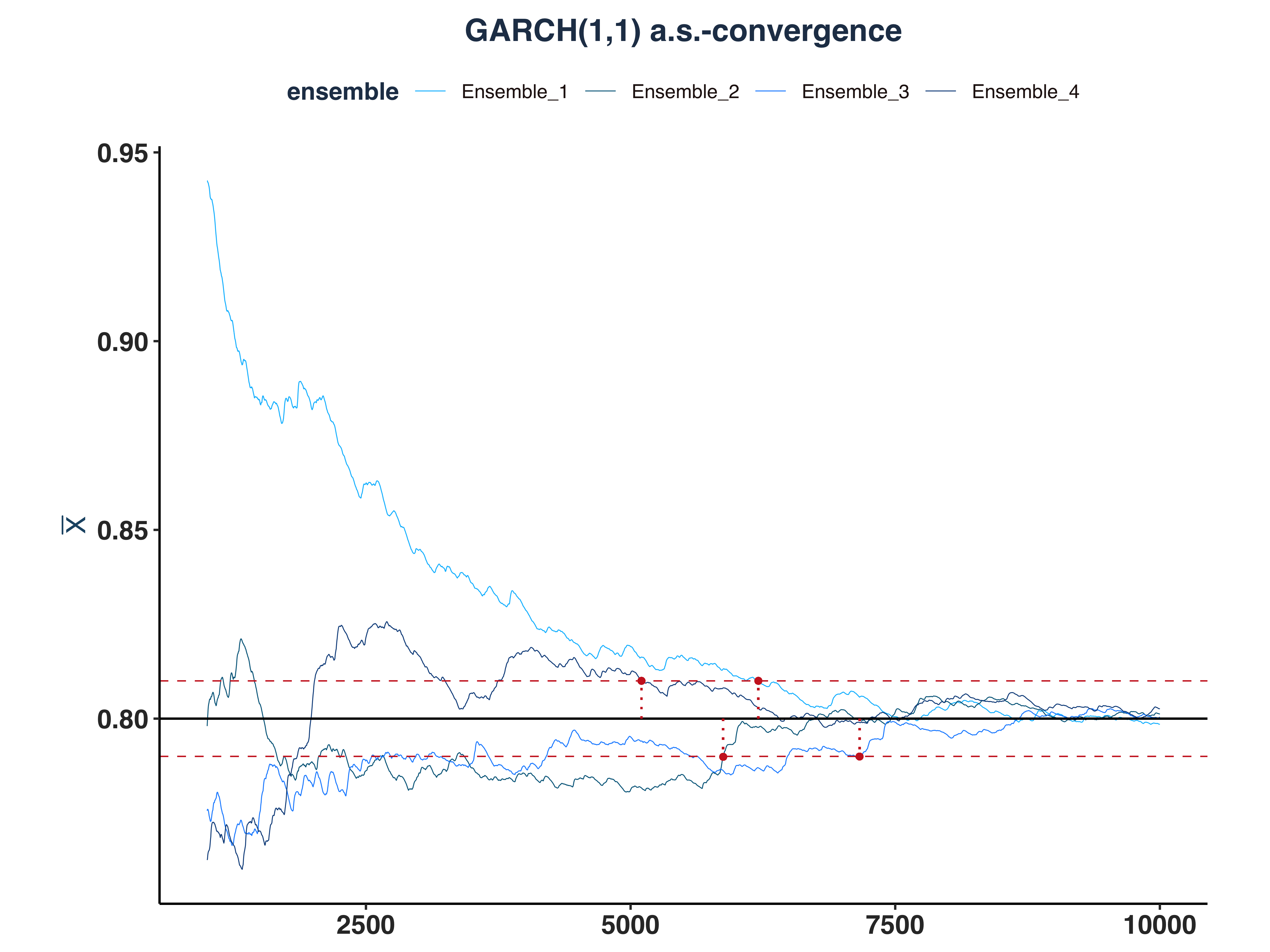
For GARCH(1,1), all of the realized conditional volatility are a.s.-converged
4. VaR 5% a.s.-convergence
1
2
3
4
5
6
7
|
# Since the first few hundreds means are so big, I cut them off for better visibility
all_var_as_conv_plt <- plot_convergence(mean_qt[1000:10000,], n_idx_var,
                                        "VaR 5%", "all", eps, mu = mu_var)

ggsave("Plots/All_VaR_5pct_as_convergence.pdf", all_var_as_conv_plt,
       width = 8, height = 6, dpi = 300)
all_var_as_conv_plt
|
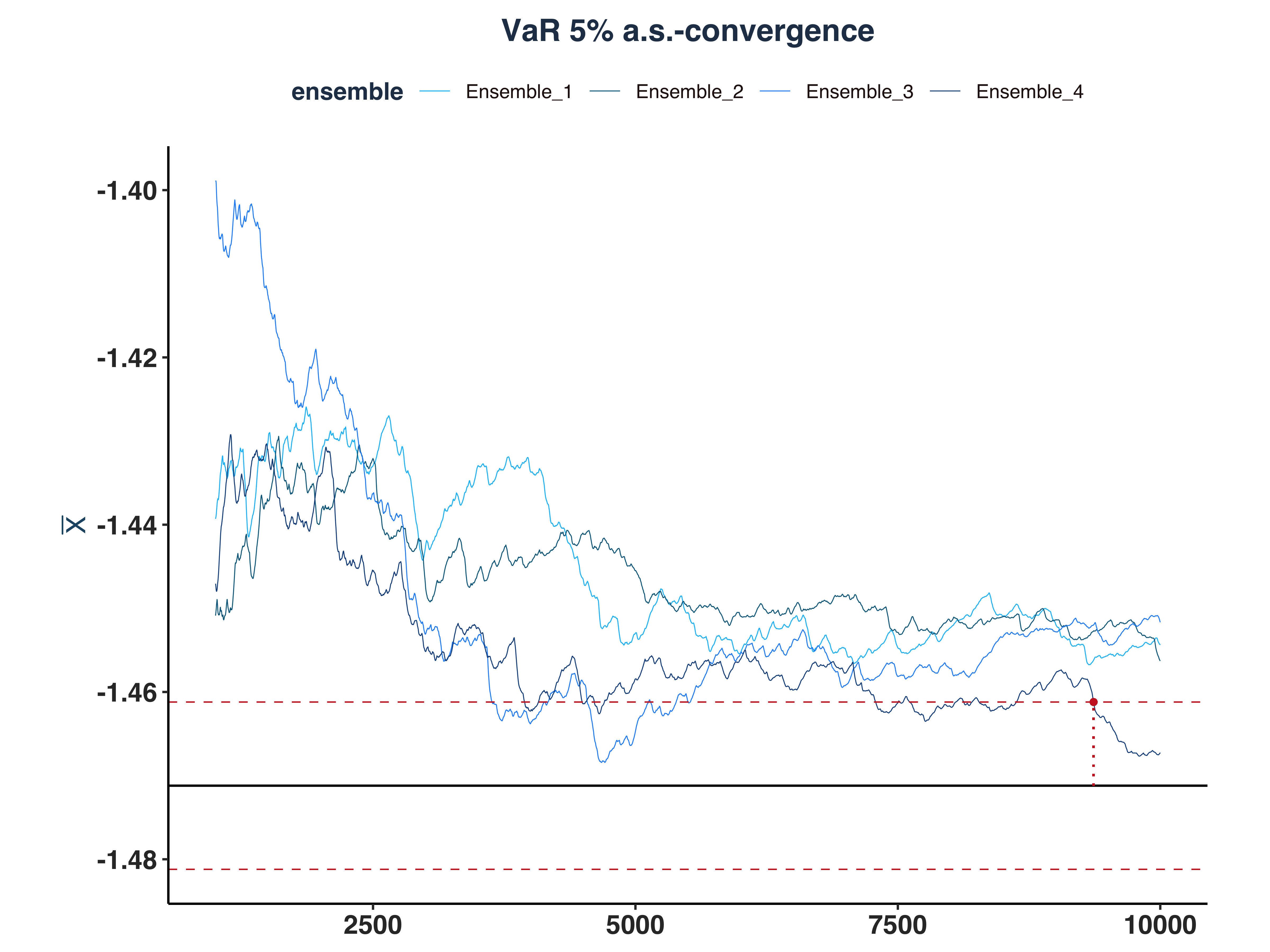
As we can see, only 1 ensemble converged.
5. ES 5% a.s.-convergence
1
2
3
4
5
6
7
|
# Since the first few hundreds means are so big, I cut them off for better visibility
all_es_as_conv_plt <- plot_convergence(mean_et[1000:10000,], n_idx_es,
                                    "ES 5%", "all", eps, mu = mu_es)

ggsave("Plots/All_ES_5pct_as_convergence.pdf", all_es_as_conv_plt,
       width = 8, height = 6, dpi = 300)
all_es_as_conv_plt
|
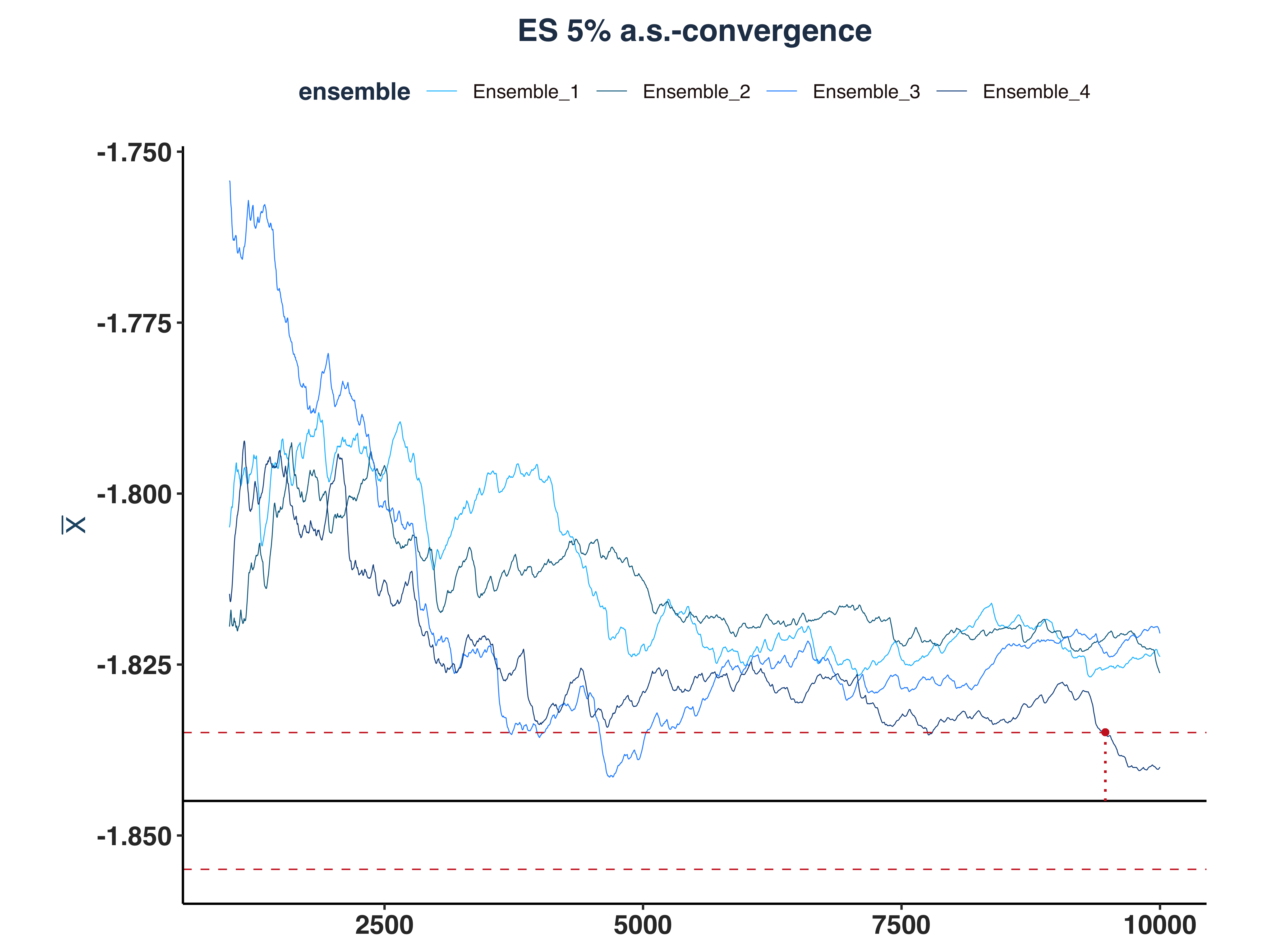
As we can see, only 1 ensemble converged.
f. Convergence in Probability#
i. Simulate Data#
Let’s simulate 200 ensemble and calculate the convergence probabilities accordingly.
 1
 2
 3
 4
 5
 6
 7
 8
 9
10
11
12
13
14
15
16
17
18
19
20
21
22
23
24
25
26
27
28
29
30
|
# Simulate the time series
set.seed(1340)
T_obs <- 10000
n_ens <- 200
sta_ts_wn <- ARMA.sim(T_obs, 0,0,0, ensembles = n_ens)
sta_ts_ar1 <- ARMA.sim(T_obs, 0.8,0,0.8, ensembles = n_ens)
sta_ts_garch11 <- GARCH.sim(T_obs, 0.04, 0.05, 0.9, ensembles = n_ens)
sta_ts_eq <- VaR.ES.sim(T_obs, 0.05, 0.04, 0.05, 0.9, ensembles = n_ens)

# Compute sequence of averages
mean_wn <- as.data.frame(apply(sta_ts_wn, 2, \(x) cumsum(x)/seq_along(x)))
mean_ar1 <- as.data.frame(apply(sta_ts_ar1, 2, \(x) cumsum(x)/seq_along(x)))
mean_g11 <- as.data.frame(apply(sta_ts_garch11$sigma.2, 2, \(x) cumsum(x)/seq_along(x)))
mean_qt <- as.data.frame(apply(sta_ts_eq$q_t, 2, \(x) cumsum(x)/seq_along(x)))
mean_et <- as.data.frame(apply(sta_ts_eq$e_t, 2, \(x) cumsum(x)/seq_along(x)))

# Compute p_T
eps <- 0.01
mu_var <- sqrt(0.8)*qnorm(0.05, 0, 1)
mu_es <- sqrt(0.8)*(-dnorm(qnorm(0.05, 0, 1), 0, 1) / 0.05)
prob_dev_wn_dt <- apply(abs(mean_wn-0), 1, \(x) {mean(x>eps)})
prob_dev_ar1_dt <- apply(abs(mean_ar1-4), 1, \(x) {mean(x>eps)})
prob_dev_g11_dt <- apply(abs(mean_g11-0.8), 1, \(x) {mean(x>eps)})
prob_dev_qt_dt <- apply(abs(mean_qt-mu_var), 1, \(x) {mean(x>eps)})
prob_dev_et_dt <- apply(abs(mean_et-mu_es), 1, \(x) {mean(x>eps)})

# Set names
list2env(lapply(mget(c("prob_dev_wn_dt", "prob_dev_ar1_dt", "prob_dev_g11_dt",
                       "prob_dev_qt_dt", "prob_dev_et_dt")),
                \(x) setNames(x, "Ensemble_1")), envir = .GlobalEnv)
|
1
|
## <environment: R_GlobalEnv>
|
1
2
3
4
5
|
# Create plot data
list2env(lapply(mget(c("prob_dev_wn_dt", "prob_dev_ar1_dt", "prob_dev_g11_dt",
                       "prob_dev_qt_dt", "prob_dev_et_dt")),
                \(x) data.frame(Index = seq_len(T_obs), Ensemble_1 = x)),
         envir = .GlobalEnv)
|
1
|
## <environment: R_GlobalEnv>
|
1
2
|
# Print out a series to double-check
tail(prob_dev_g11_dt,10)
|
 1
 2
 3
 4
 5
 6
 7
 8
 9
10
11
|
##       Index Ensemble_1
## 9991   9991       0.39
## 9992   9992       0.39
## 9993   9993       0.39
## 9994   9994       0.39
## 9995   9995       0.39
## 9996   9996       0.39
## 9997   9997       0.39
## 9998   9998       0.39
## 9999   9999       0.39
## 10000 10000       0.39
|
ii. Plot the Convergence in Probability#
1. White Noise Kernel Density
1
2
3
4
5
6
|
wn_ip_conv_plt <- plot_convergence(prob_dev_wn_dt, NULL, "White Noise", "Ensemble_1",
                                   eps = 0, mu = 0) # (eps,mu)=(0,0) values a specifically for in probability convergence

ggsave("Plots/White_Noise_ip_convergence.pdf", wn_ip_conv_plt,
       width = 8, height = 6, dpi = 300)
wn_ip_conv_plt
|
2. AR(1) Kernel Density
1
2
3
4
5
6
|
ar1_ip_conv_plt <- plot_convergence(prob_dev_ar1_dt, NULL, "AR(1)", "Ensemble_1",
                                    eps=0, mu = 0)

ggsave("Plots/AR1_ip_convergence.pdf", ar1_ip_conv_plt,
       width = 8, height = 6, dpi = 300)
ar1_ip_conv_plt
|
3. GARCH(1,1) Kernel Density
1
2
3
4
5
6
|
g11_ip_conv_plt <- plot_convergence(prob_dev_g11_dt, NULL, "GARCH(1,1)",
                                    "Ensemble_1", eps = 0, mu = 0)

ggsave("Plots/GARCH11_ip_convergence.pdf", g11_ip_conv_plt,
       width = 8, height = 6, dpi = 300)
g11_ip_conv_plt
|
4. VaR 5% Kernel Density
1
2
3
4
5
6
|
var_ip_conv_plt <- plot_convergence(prob_dev_qt_dt, NULL, "VaR 5%", "Ensemble_1",
                                    eps = 0, mu = 0)

ggsave("Plots/VaR_5pct_ip_convergence.pdf", var_ip_conv_plt,
       width = 8, height = 6, dpi = 300)
var_ip_conv_plt
|
5. ES 5% Kernel Density
1
2
3
4
5
6
|
es_ip_conv_plt <- plot_convergence(prob_dev_et_dt, NULL, "ES 5%", "Ensemble_1",
                                   eps = 0, mu = 0)

ggsave("Plots/ES_5pct_ip_convergence.pdf", es_ip_conv_plt,
       width = 8, height = 6, dpi = 300)
es_ip_conv_plt
|
g. Simulate 200 Ensembles and Find \(\bar{n}(\varepsilon=0.01, \omega)\)#
i. Simulate and Compute \(\bar{n}\)#
 1
 2
 3
 4
 5
 6
 7
 8
 9
10
11
12
13
14
15
16
17
18
19
20
21
22
23
24
25
26
27
28
29
30
31
32
33
34
35
36
37
38
39
40
41
42
43
44
45
46
47
48
49
50
51
52
53
54
55
56
57
58
59
|
# Define file paths
data_files <- list(
  wn = "Data/sta_ts_wn_dt.rds",
  ar1 = "Data/sta_ts_ar1_dt.rds",
  garch11 = "Data/sta_ts_garch11_dt.rds",
  qt = "Data/sta_ts_qt_dt.rds",
  et = "Data/sta_ts_et_dt.rds"
)

# Check if all files exist
all_files_exist <- all(sapply(data_files, file.exists))

if (!all_files_exist) {
  # Simulate the time series
  set.seed(1340)
  T_obs <- 100000
  n_ens <- 200
  sta_ts_wn <- ARMA.sim(T_obs, 0,0,0, ensembles = n_ens)
  sta_ts_ar1 <- ARMA.sim(T_obs, 0.8,0,0.8, ensembles = n_ens)
  sta_ts_garch11 <- GARCH.sim(T_obs, 0.04, 0.05, 0.9, ensembles = n_ens)
  sta_ts_eq <- VaR.ES.sim(T_obs, 0.05, 0.04, 0.05, 0.9, ensembles = n_ens)

  # Convert simulated data to data.table
  sta_ts_wn_dt <- as.data.table(sta_ts_wn)
  sta_ts_ar1_dt <- as.data.table(sta_ts_ar1)
  sta_ts_garch11_dt <- as.data.table(sta_ts_garch11$sigma.2)
  sta_ts_qt_dt <- as.data.table(sta_ts_eq$q_t)
  sta_ts_et_dt <- as.data.table(sta_ts_eq$e_t)

  # Set column names
  col_names <- paste0("Ensemble_", 1:n_ens)
  setnames(sta_ts_wn_dt, col_names)
  setnames(sta_ts_ar1_dt, col_names)
  setnames(sta_ts_garch11_dt, col_names)
  setnames(sta_ts_qt_dt, col_names)
  setnames(sta_ts_et_dt, col_names)

  # Save datasets to disk
  saveRDS(sta_ts_wn_dt, file = data_files$wn)
  saveRDS(sta_ts_ar1_dt, file = data_files$ar1)
  saveRDS(sta_ts_garch11_dt, file = data_files$garch11)
  saveRDS(sta_ts_qt_dt, file = data_files$qt)
  saveRDS(sta_ts_et_dt, file = data_files$et)
} else {
  # Load saved datasets
  sta_ts_wn_dt <- readRDS(data_files$wn)
  sta_ts_ar1_dt <- readRDS(data_files$ar1)
  sta_ts_garch11_dt <- readRDS(data_files$garch11)
  sta_ts_qt_dt <- readRDS(data_files$qt)
  sta_ts_et_dt <- readRDS(data_files$et)
}

# Compute sequence of averages using data.table syntax
# apply to all column, please advise https://cran.r-project.org/web/packages/data.table/vignettes/datatable-sd-usage.html
mean_wn <- sta_ts_wn_dt[, lapply(.SD, \(x) cumsum(x)/seq_along(x))]
mean_ar1 <- sta_ts_ar1_dt[, lapply(.SD, \(x) cumsum(x)/seq_along(x))]
mean_g11 <- sta_ts_garch11_dt[, lapply(.SD, \(x) cumsum(x)/seq_along(x))]
mean_qt <- sta_ts_qt_dt[, lapply(.SD, \(x) cumsum(x)/seq_along(x))]
mean_et <- sta_ts_et_dt[, lapply(.SD, \(x) cumsum(x)/seq_along(x))]
|
 1
 2
 3
 4
 5
 6
 7
 8
 9
10
11
12
13
14
15
16
17
18
19
20
21
22
23
24
25
|
# Compute deviations
eps <- 0.01
mu_var <- sqrt(0.8)*qnorm(0.05, 0, 1)
mu_es <- sqrt(0.8)*(-dnorm(qnorm(0.05, 0, 1), 0, 1) / 0.05)

abs_dev_wn_dt <- mean_wn[, lapply(.SD, \(x) abs(x - 0))]      # mu=0
abs_dev_ar1_dt <- mean_ar1[, lapply(.SD, \(x) abs(x - 4))]    # mu=4
abs_dev_g11_dt <- mean_g11[, lapply(.SD, \(x) abs(x - 0.8))]  # mu=0.8
abs_dev_qt_dt <- mean_qt[, lapply(.SD, \(x) abs(x - mu_var))] # mu=-1.4712
abs_dev_et_dt <- mean_et[, lapply(.SD, \(x) abs(x - mu_es))]  # mu=-1.8449

# Add Index column for plotting
mean_wn[, Index := .I]
mean_ar1[, Index := .I]
mean_g11[, Index := .I]
mean_qt[, Index := .I]
mean_et[, Index := .I]

# Reorder columns to put Index first
col_names <- paste0("Ensemble_", 1:ncol(sta_ts_wn_dt))
setcolorder(mean_wn, c("Index", col_names))
setcolorder(mean_ar1, c("Index", col_names))
setcolorder(mean_g11, c("Index", col_names))
setcolorder(mean_qt, c("Index", col_names))
setcolorder(mean_et, c("Index", col_names))
|
 1
 2
 3
 4
 5
 6
 7
 8
 9
10
11
12
13
14
15
16
17
18
19
20
21
22
23
24
25
|
# Create a single list containing all data
sta_ts_all_dt <- list(
  wn = abs_dev_wn_dt,
  ar1 = abs_dev_ar1_dt,
  g11 = abs_dev_g11_dt,
  qt = abs_dev_qt_dt,
  et = abs_dev_et_dt
)

n_idx_ls <- lapply(sta_ts_all_dt, \(dt) {
  dt[, lapply(.SD, \(x) {
    rs <- rev(cumsum(rev(as.numeric(x > eps))))
    idx <- max(which(rs == 1))
    if(idx == length(x)) NA_integer_ else idx
  })]
})

# Check convergence
n_non_conv <- sapply(n_idx_ls, \(dt) dt[, sum(sapply(.SD, is.na))])

if(sum(n_non_conv) > 0) {
  cat("Non-converged ensembles exist")
} else {
  cat("All ensembles converged")
}
|
1
|
## Non-converged ensembles exist
|
1
2
3
4
5
6
|
data.table(
  Series = names(n_non_conv),
  Non_Converged = as.numeric(n_non_conv),
  Total_Ensembles = sapply(n_idx_ls, ncol),
  Convergence_Rate = round((1 - as.numeric(n_non_conv) / sapply(n_idx_ls, ncol)) * 100, 2)
)
|
1
2
3
4
5
6
7
|
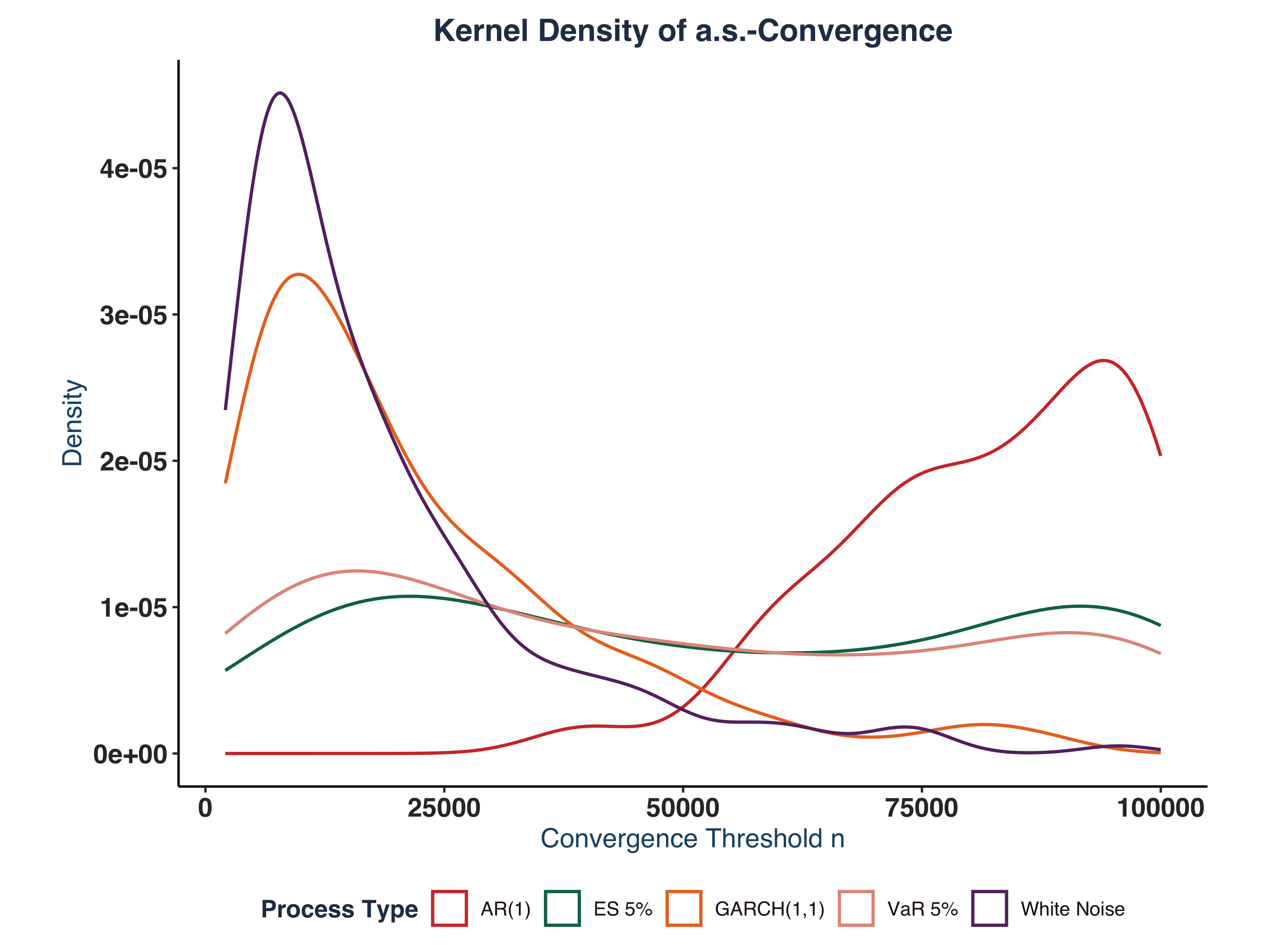
##    Series Non_Converged Total_Ensembles Convergence_Rate
##    <char>         <num>           <int>            <num>
## 1:     wn             0             200              100
## 2:    ar1           118             200               41
## 3:    g11             2             200               99
## 4:     qt            76             200               62
## 5:     et           126             200               37
|
ii. Plot Kernel Density#
 1
 2
 3
 4
 5
 6
 7
 8
 9
10
11
12
13
14
15
16
17
18
19
20
21
22
23
24
25
26
27
28
29
30
31
32
33
34
|
# Create a mapping for proper names
process_names <- c("wn" = "White Noise", "ar1" = "AR(1)", "g11" = "GARCH(1,1)",
                   "qt" = "VaR 5%", "et" = "ES 5%")

# Combine all series
plt_dt <- rbindlist(lapply(names(n_idx_ls), \(name) {
  data.table(n = as.vector(t(n_idx_ls[[name]])),
             process = process_names[name])
}))

# Create the plot with proper labels
ts_colors <- c("White Noise" = "#663171FF",
           "AR(1)" = "#CF3A36FF",
           "GARCH(1,1)" = "#EA7428FF",
           "VaR 5%" = "#E2998AFF",
           "ES 5%" = "#0C7156FF")
dens_plt <- ggplot(plt_dt, aes(x = n)) +
  geom_density(aes(color = process), linewidth = 0.7) +
  scale_fill_manual(values = ts_colors)+
  scale_color_manual(values = ts_colors)+
  theme(panel.grid.major = element_blank(),
        panel.grid.minor = element_blank(),
        panel.border = element_blank(),
        panel.background = element_blank(),
        legend.position = "bottom") +
  global_fonts+
  labs(title = "Kernel Density of a.s.-Convergence",
       x = "Convergence Threshold n",
       y = "Density",
       color = "Process Type")

ggsave("Plots/Convergence_kernel_density.pdf", dens_plt,
       width = 8, height = 6, dpi = 300)
dens_plt
|
Exercise 3 - Forecasting Exercise#
a. Pseudo-out-of Sample One-step Ahead Forecast#
i. Setup Forecast#
First, we split the Coca-Cola (KO) stock log returns into two datasets: train_dt (70%) and test_dt (30%).
 1
 2
 3
 4
 5
 6
 7
 8
 9
10
11
12
13
14
15
16
17
18
19
20
21
22
23
24
25
26
27
28
29
30
31
32
|
# Model Setup ----
# 1. Crawl More data
if (!file.exists("Data/ex3_price_dt.rds")) {
  # Download Data
  ex3_pr_dt <- tq_get("KO",get = "stock.prices", from = "1990-01-01", to = "2025-08-09")
  # Save model data
  saveRDS(ex3_pr_dt, file = "Data/ex3_price_dt.rds")
} else {
  # Access saved stock data
  ex3_pr_dt <- readRDS("Data/ex3_price_dt.rds")
}
# Prepare return data
ex3_ret_dt <- prep_return_dt(ex3_pr_dt)
# Extract different frequencies
ex3_daily_dt <- ex3_ret_dt$daily

# 2. Train Test split
ex3_daily_dt <- data.table(ex3_daily_dt)
n_obs <- nrow(ex3_daily_dt)
train_idx <- 1:floor(n_obs*0.7)
train_dt <- ex3_daily_dt[train_idx, c("date","logret")]
test_dt <- ex3_daily_dt[!train_idx, c("date","logret")]

# 2. Config
control.solnp <- list(rho        = 1,
                      outer.iter = 600,
                      inner.iter = 800,
                      delta      = 1e-7,
                      tol        = 1e-6)

# Print out lengths
sprintf("Number of observation in Train Dataset: %d", nrow(train_dt))
|
1
|
## [1] "Number of observation in Train Dataset: 6276"
|
1
|
sprintf("Number of observation in Test Dataset: %d", nrow(test_dt))
|
1
|
## [1] "Number of observation in Test Dataset: 2690"
|
ii. Model Selection#
Based on the results from Exercise 1.b, we observe that GARCH(1,1) is the best candidate for our problem. Following previouse researches of Nkrumah, M. A. (2025), Enkhtur, A. (2022), Yatawara, K. C. M. R. A. B. (2023), Sjöholm, S. (2015), and So, M. K. P., Chu, A. M. Y., Lo, C. C. Y., & Ip, C. Y. (2021), we will compare the performance among three models: GJR-GARCH-N, EGARCH, and GARCH-t.
 1
 2
 3
 4
 5
 6
 7
 8
 9
10
11
12
13
14
15
16
17
18
19
20
21
22
23
24
25
26
27
|
# Get bounds
mdl_name <-  "GJR-GARCH-N"
bounds <- get_garch_bounds(mdl_name, c(1,1))

if (!file.exists("Data/ex3_gjrgn_mdl.rds")) {
# Estimate GJR-GARCH-N
ex3_gjr_mdl <- estimate_garch_dynamic(
    y = train_dt[["logret"]],
    n_starts = 20,
    garch_order = c(1,1),
    model_type = "GJR-GARCH-N",
    distribution = "norm",
    lower_bounds = bounds$lower, upper_bounds = bounds$upper,
    loglik_func = Likelihood.GARCH,
    ineq_constraints = Inequality.constraints.GARCH,
    custom_control = control.solnp
  )

  # Save results
  saveRDS(ex3_gjr_mdl, file = "Data/ex3_gjrgn_mdl.rds")
} else {
  # Access saved  data
  ex3_gjr_mdl <- readRDS("Data/ex3_gjrgn_mdl.rds")
}

# Check best log-likelihood
# sprintf("Best LLH rugarch %s: %.2f", mdl_name, ex3_gjr_mdl$best_estimates$rugarch["LogL"])
|
 1
 2
 3
 4
 5
 6
 7
 8
 9
10
11
12
13
14
15
16
17
18
19
20
21
22
23
24
25
26
27
|
# Get bounds
mdl_name2 <-  "EGARCH"
bounds2 <- get_garch_bounds(mdl_name2, c(1,1))

if (!file.exists("Data/ex3_eg_mdl.rds")) {
# Estimate GJR-GARCH-N
ex3_eg_mdl <- estimate_garch_dynamic(
    y = train_dt[["logret"]],
    n_starts = 20,
    garch_order = c(1,1),
    model_type = mdl_name2,
    distribution = "sstd",
    lower_bounds = bounds2$lower, upper_bounds = bounds2$upper,
    loglik_func = Likelihood.GARCH,
    ineq_constraints = Inequality.constraints.GARCH,
    custom_control = control.solnp
  )

  # Save results
  saveRDS(ex3_eg_mdl, file = "Data/ex3_eg_mdl.rds")
} else {
  # Access saved  data
  ex3_eg_mdl <- readRDS("Data/ex3_eg_mdl.rds")
}

# Check best log-likelihood
# sprintf("Best LLH rugarch %s: %.2f", mdl_name2, ex3_eg_mdl$best_estimates$rugarch["LogL"])
|
 1
 2
 3
 4
 5
 6
 7
 8
 9
10
11
12
13
14
15
16
17
18
19
20
21
22
23
24
|
# Get bounds
mdl_name3 <-  "GARCH-t"
bounds3 <- get_garch_bounds(mdl_name3, c(1,1))

if (!file.exists("Data/ex3_gt_mdl.rds")) {
# Estimate GJR-GARCH-N
ex3_gt_mdl <- estimate_garch_dynamic(
    y = train_dt[["logret"]],
    n_starts = 20,
    garch_order = c(1,1),
    model_type = mdl_name3,
    distribution = "std",
    lower_bounds = bounds3$lower, upper_bounds = bounds3$upper,
    loglik_func = Likelihood.GARCH,
    ineq_constraints = Inequality.constraints.GARCH,
    custom_control = control.solnp
  )

  # Save results
  saveRDS(ex3_gt_mdl, file = "Data/ex3_gt_mdl.rds")
} else {
  # Access saved  data
  ex3_gt_mdl <- readRDS("Data/ex3_gt_mdl.rds")
}
|
 1
 2
 3
 4
 5
 6
 7
 8
 9
10
11
12
13
14
|
# Create comparison table
model_comparison <- data.frame(
  Model = c("GJR-GARCH-N", "EGARCH", "GARCH-t"),
  Best_LogLikelihood = c(
    max(ex3_gjr_mdl$best_estimates$rugarch["LogL"],
        ex3_gjr_mdl$best_estimates$solnp["LogL"], na.rm = TRUE),
    max(ex3_eg_mdl$best_estimates$rugarch["LogL"],
        ex3_eg_mdl$best_estimates$solnp["LogL"], na.rm = TRUE),
    max(ex3_gt_mdl$best_estimates$rugarch["LogL"],
        ex3_gt_mdl$best_estimates$solnp["LogL"], na.rm = TRUE)
  )
)

print(model_comparison, row.names = FALSE)
|
1
2
3
4
|
##        Model Best_LogLikelihood
##  GJR-GARCH-N          -18446.74
##       EGARCH          -18662.05
##      GARCH-t          -18246.79
|
The result suggests that GARCH-t performs slightly better than the other two in terms of best-fit log-likelihood.
iii. Test Out-of-sample Estimate#
After collecting the best fitted model from solnp solver, we can test the best estimated parameters out-of-sample.
  1
  2
  3
  4
  5
  6
  7
  8
  9
 10
 11
 12
 13
 14
 15
 16
 17
 18
 19
 20
 21
 22
 23
 24
 25
 26
 27
 28
 29
 30
 31
 32
 33
 34
 35
 36
 37
 38
 39
 40
 41
 42
 43
 44
 45
 46
 47
 48
 49
 50
 51
 52
 53
 54
 55
 56
 57
 58
 59
 60
 61
 62
 63
 64
 65
 66
 67
 68
 69
 70
 71
 72
 73
 74
 75
 76
 77
 78
 79
 80
 81
 82
 83
 84
 85
 86
 87
 88
 89
 90
 91
 92
 93
 94
 95
 96
 97
 98
 99
100
101
102
103
104
105
106
107
108
109
110
111
112
113
114
115
116
117
118
119
120
121
122
123
124
125
126
127
128
129
130
131
132
133
134
135
136
137
138
139
140
141
142
143
144
145
146
147
|
## Setup for OOS Forecast ----
# Extract best estimated parameters
best_gt_pars <- vector_to_named_pars(ex3_gt_mdl$best_estimates$solnp[1:5],
                                     model_type = "GARCH-t", distribution = "std")
names(best_gt_pars)[5] <- "shape"

# Pre-allocate fitted parameters
n_test <- nrow(test_dt)
n_oos <- n_test+250
ex3_gt_pars_dt <- data.table(
  mu = rep(best_gt_pars$mu, n_test + 1),
  omega = rep(best_gt_pars$omega, n_test + 1),
  alpha1 = rep(best_gt_pars$alpha1, n_test + 1),
  beta1 = rep(best_gt_pars$beta1, n_test + 1),
  shape = rep(best_gt_pars$shape, n_test + 1)
)

if (!file.exists("Data/ex3_gt_pars_dt.rds") &&
    !file.exists("Data/tracking_df.rds") &&
    !file.exists("Data/oos_rlt.rds")) {
  ## Pre-allocate a result dataset
  oos_rlt <- ex3_daily_dt[(n_obs-n_oos+1):n_obs, # combine last 250 train + all test
                        .(date = date, act_ret = logret, prd_var = 0.0,
                          prd_vol = 0.0, std_res = 0.0, log_lik = 0.0)]

  ## Initialize tracking dataframe ----
  tracking_df <- data.frame(
    step = integer(0),
    issue_type = character(0),
    message = character(0),
    stringsAsFactors = FALSE
  )

  ## Main Estimate Loop ----
  for (i in seq_len(n_test)) {
    # Create specs using parameters from step t
    spec <- ugarchspec(
      variance.model = list(model = "sGARCH", garchOrder = c(1,1)),
      mean.model = list(armaOrder = c(0,0)),
      distribution.model = "std",
      start.pars = as.list(ex3_gt_pars_dt[i])
    )

    # Extract sliding window
    wd_dt <- oos_rlt[seq(from = i, length.out = 250), act_ret]

    # Fit model with error handling
    fit <- tryCatch({
      ugarchfit(spec, data = wd_dt)
    }, error = function(e) {
      # Log error to dataframe
      tracking_df <- rbind(tracking_df, data.frame(
        step = i,
        issue_type = "fit_error",
        message = e$message,
        stringsAsFactors = FALSE
      ))
      return(NULL)
    }, warning = function(w) {
      # Log warning to dataframe
      tracking_df <- rbind(tracking_df, data.frame(
        step = i,
        issue_type = "fit_warning",
        message = w$message,
        stringsAsFactors = FALSE
      ))
      suppressWarnings(ugarchfit(spec, data = wd_dt))
    })

    # Check if fit was successful
    if (is.null(fit)) {
      # Carry forward previous parameters (no update)
      ex3_gt_pars_dt[i + 1] <- ex3_gt_pars_dt[i]

      # Set forecast outputs to NA
      oos_rlt[i + 250, `:=`(
        log_lik = NA_real_,
        prd_vol = NA_real_,
        std_res = NA_real_
      )]

      next  # Skip to next iteration
    }

    # Check convergence status (additional check)
    if (rugarch::convergence(fit) != 0) {
      tracking_df <- rbind(tracking_df, data.frame(
        step = i,
        issue_type = "convergence_issue",
        message = paste("Convergence code:", rugarch::convergence(fit)),
        stringsAsFactors = FALSE
      ))
    }

    # Forecast one step ahead
    forecast <- tryCatch({
      ugarchforecast(fit, n.ahead = 1)
    }, error = function(e) {
      # Log forecast error
      tracking_df <- rbind(tracking_df, data.frame(
        step = i,
        issue_type = "forecast_error",
        message = e$message,
        stringsAsFactors = FALSE
      ))
      return(NULL)
    })

    if (is.null(forecast)) {
      # If forecast fails, carry forward parameters but set outputs to NA
      ex3_gt_pars_dt[i + 1] <- ex3_gt_pars_dt[i]
      oos_rlt[i + 250, `:=`(log_lik = NA_real_,prd_vol = NA_real_,std_res = NA_real_)]
      next
    }

    # Extract forecast outputs
    prd_mu <- rugarch::fitted(forecast)[1]
    oos_rlt[i + 250, `:=`(
      log_lik = -likelihood(fit),
      prd_vol = rugarch::sigma(forecast)[1],
      std_res = (act_ret - prd_mu) / rugarch::sigma(forecast)[1]
    )]

    # Store fitted parameters for NEXT iteration
    cf <- coef(fit)
    ex3_gt_pars_dt[i + 1, `:=`(
      mu = cf["mu"],
      omega = cf["omega"],
      alpha1 = cf["alpha1"],
      beta1 = cf["beta1"],
      shape = cf["shape"]
    )]
  }

  # Save results
  saveRDS(ex3_gt_pars_dt, file = "Data/ex3_gt_pars_dt.rds")
  saveRDS(tracking_df, file = "Data/tracking_df.rds")
  saveRDS(oos_rlt, file = "Data/oos_rlt.rds")
} else {
  # Access saved  data
  ex3_gt_pars_dt <- readRDS("Data/ex3_gt_pars_dt.rds")
  tracking_df <- readRDS("Data/tracking_df.rds")
  oos_rlt <- readRDS("Data/oos_rlt.rds")
}

## Summary Report ----
cat(paste(rep("=", 50), collapse=""),"\n")
|
1
|
## ==================================================
|
1
|
cat("GARCH ESTIMATION SUMMARY\n")
|
1
|
## GARCH ESTIMATION SUMMARY
|
1
|
cat(paste(rep("=", 50), collapse=""), "\n")
|
1
|
## ==================================================
|
1
2
3
4
5
6
|
# Overall statistics
total_issues <- nrow(tracking_df)
successful_fits <- n_test - length(which(tracking_df$issue_type == "fit_error"))
success_rate <- successful_fits / n_test * 100

cat(paste(rep("=", 50), collapse=""), "\n")
|
1
|
## ==================================================
|
1
|
cat(sprintf("Total iterations: %d\n", n_test))
|
1
|
## Total iterations: 2690
|
1
|
cat(sprintf("Successful fits: %d (%.1f%%)\n", successful_fits, success_rate))
|
1
|
## Successful fits: 2690 (100.0%)
|
1
|
cat(sprintf("Total issues logged: %d\n", total_issues))
|
1
|
## Total issues logged: 283
|
1
|
cat(paste(rep("=", 50), collapse=""), "\n")
|
1
|
## ==================================================
|
1
2
3
4
|
# Compute predicted variance `prd_var`
oos_rlt[, prd_var := prd_vol^2]
# Print a summary of the OOS result
summary(oos_rlt[251:n_oos])
|
 1
 2
 3
 4
 5
 6
 7
 8
 9
10
11
12
13
14
15
16
|
##       date               act_ret              prd_var           prd_vol
##  Min.   :2014-11-26   Min.   :-0.1017278   Min.   :0.00003   Min.   :0.00508
##  1st Qu.:2017-07-31   1st Qu.:-0.0047282   1st Qu.:0.00006   1st Qu.:0.00796
##  Median :2020-04-01   Median : 0.0004840   Median :0.00009   Median :0.00922
##  Mean   :2020-04-01   Mean   : 0.0002969   Mean   :0.00014   Mean   :0.01065
##  3rd Qu.:2022-11-30   3rd Qu.: 0.0058709   3rd Qu.:0.00014   3rd Qu.:0.01176
##  Max.   :2025-08-08   Max.   : 0.0627831   Max.   :0.00518   Max.   :0.07197
##                                            NA's   :283       NA's   :283
##     std_res             log_lik
##  Min.   :-11.58449   Min.   :-950.8
##  1st Qu.: -0.56765   1st Qu.:-856.7
##  Median : -0.00092   Median :-828.8
##  Mean   : -0.03292   Mean   :-822.9
##  3rd Qu.:  0.54034   3rd Qu.:-800.4
##  Max.   :  6.33997   Max.   :-653.2
##  NA's   :283         NA's   :283
|
Note: My current approach involves using the entire train_dt to obtain the best parameter estimates for the first one-step ahead forecast, then employing a 250-day window for re-estimating parameters. The question arose as it required more than 6,000 observation in train_dt to achieve convergence; thus, the 250 data points appears insufficient for the re-estimation.
However, the practical evidence in my result indicates that there remains 10.52 of unconverged forecasts. As a result, I believe increasing the window size to 6,000 (or at least 4,000 as you suggested) would be a potential solution for this. Please kindly let me know if my understanding is correct and the solution is feasible.
iv. Why modles in 1b) are valid candidates?#
Based on the following criteria, one may conclude the validity of a GARCH-type candidate model for conditional volatility forecasting:
- Evidence of Excessive Kurtosis & Skewness, tested using Jarque–Bera Test and/or D’Agostino skewness test, or Shapiro-Wilk test.
- Existence of Volatility Clustering, examined via time series plots of squared returns, ACF plots of squared/absolute returns, or tested using Ljung-Box Test
- Presence of Conditional Heteroskedasticity verified by ARCH-LM Test.
- Serial Correlation pattern: significant correlation in squared/absolute returns but no correlation in raw returns (tested via Ljung-Box tests).
- Indication of Levarage Effect, which produces higher volatility after negative shocks, or quantile-based volatility comparisons.
These properties validate GARCH-N, GARCH-t, EGARCH, and GJR-GARCH-N as potential candidates for conditional volatility forecasting.
v. Why is the EGARCH diffcult to work with?#
There exists multiple challenges when working with EGARCH model, including:
- The model structure is non-linear logarithmic, implying no closed-form solution:
$$
h_t = \omega + \beta h_{t-1} + \alpha \epsilon_{t-1} + \gamma \left(|\epsilon_{t-1}| - \mathbb{E}|\epsilon_{t-1}|\right), \quad h_t = \ln(\sigma_t^2)
$$
- The estimation process involves recursive computation of
\(\theta\), increasing the complexity of computation and the risk of explosion, i.e. \(\theta\) is estimated by evaluating:
$$
h_t(\theta) = \omega - \gamma \mathbb{E}|\epsilon_t| + \alpha \epsilon_{t-1}(\theta) + \gamma |\epsilon_{t-1}(\theta)| + \beta h_{t-1}(\theta)
$$
- As a consequence, the resulting log-likelihood function poses a huge numerical optimization challenge due to its complexity in gradient calculation. The Log-likelihood function is given by:
$$
\mathcal{L}(\theta) = -\sum_{t=k+1}^{T} h_t(\theta) - \frac{1}{2} \sum_{t=k+1}^{T} X_t^2 \exp{-2h_t(\theta)}
$$
- This also leads to large deviations in gradient computation in response to small changes in input
\(\theta\) as it is amplified by chain rule.
- The asymmetric function also contributes to the complexity of the optimization problem because it is non-differentiable at zero:
$$
g(\epsilon_{t-1}) = \begin{cases}
(\alpha + \gamma) - \gamma\mathbb E|\epsilon_{t-1}| & \epsilon_{t-1}\geq 0 \
(\alpha - \gamma) - \gamma\mathbb E|\epsilon_{t-1}| & \epsilon_{t-1} < 0
\end{cases}
$$
For these reasons, the EGARCH model frequently suffers from convergence issues during estimation and faces high sensitivity to starting values. This model consequently demands a high level of numerical precision while optimizing, which makes it less attractive despite of theoretical advantages.
b. Explain One-step Ahead Forecast#
i. GARCH-N Model#
- Model specification:
- Returns:
\(r_t = \mu_t + \varepsilon_t\) where \(\varepsilon_t = \sigma_t\eta_t, \ \eta_t \sim \mathcal{N}(0,1)\)
- Conditional Variance:
\(\sigma_t^2 = \omega + \alpha\varepsilon_{t-1}^2 +\beta\sigma_{t-1}^2\)
- One-step ahead variance forecast:
\(\mathbb E[\sigma_{t+1}^2 \mid \mathcal{F}_{t}] = \omega + \alpha\varepsilon_{t}^2+\beta\sigma_{t}^2\)
- One-step ahead return forecast:
\(\mathbb E[r_{t+1} \mid \mathcal{F}_{t}] = \mathbb E[\mu_{t+1} \mid \mathcal{F}_{t}]\)
- Information set:
\(\mathcal{F}_{t} = \{r_t, r_{t-1},..., \varepsilon_{t}^2, \varepsilon_{t-1}^2,...,\sigma_{t}^2, \sigma_{t-1}^2,...\}\)
ii. GARCH-t Model#
- Model specification:
- Returns:
\(r_t = \mu_t + \varepsilon_t\) where \(\varepsilon_t = \sigma_t\eta_t, \ \eta_t \sim t_\nu\)
- Conditional Variance:
\(\sigma_t^2 = \omega + \alpha\varepsilon_{t-1}^2 +\beta\sigma_{t-1}^2\)
- One-step ahead variance forecast:
\(\mathbb E[\sigma_{t+1}^2 \mid \mathcal{F}_{t}] = \omega + \alpha\varepsilon_{t}^2 +\beta\sigma_{t}^2\)
- One-step ahead return forecast:
\(\mathbb E[r_{t+1} \mid \mathcal{F}_{t}] = \mathbb E[\mu_{t+1} \mid \mathcal{F}_{t}]\)
- Information set:
\(\mathcal{F}_{t} = \{r_t, r_{t-1},..., \varepsilon_{t}^2, \varepsilon_{t-1}^2,...,\sigma_{t}^2, \sigma_{t-1}^2,...\}\)
- Major distinction between GARCH-N and GARCH-t is the distribution of
\(\eta_t\), which changes from standard normal to student t distribution.
iii. GJR-GARCH-N Model#
- Model specification:
- Returns:
\(r_t = \mu_t + \varepsilon_t\) where \(\varepsilon_t = \sigma_t\eta_t, \ \eta_t \sim \mathcal{N}(0,1)\)
- Conditional Variance:
\(\sigma_t^2 = \omega + (\alpha_1 + \gamma_1 \mathbb I(\varepsilon_{t-1} < 0))\varepsilon_{t-1}^2 +\beta_1\sigma_{t-1}^2\)
- One-step ahead variance forecast:
\(\mathbb E[\sigma_{t+1}^2 \mid \mathcal{F}_{t}] = \omega + (\alpha_1 + \gamma_1 \mathbb I(\varepsilon_{t} < 0))\varepsilon_{t}^2 +\beta_1\sigma_{t}^2\)
- One-step ahead return forecast:
\(\mathbb E[r_{t+1} \mid \mathcal{F}_{t}] = \mathbb E[\mu_{t+1} \mid \mathcal{F}_{t}]\)
- Information set:
\(\mathcal{F}_{t} = \{r_t, r_{t-1},..., \varepsilon_{t}^2, \varepsilon_{t-1}^2,...,\sigma_{t}^2, \sigma_{t-1}^2,..., \mathbb I(\varepsilon_{t} < 0), \mathbb I(\varepsilon_{t-1} < 0),...\}\)
- Key difference from GARCH-N: the information set
\(\mathcal{F}_{t}\) includes the signs of current & past shock \(\mathbb I_t, \mathbb I_{t-1},...\).
c. Generate Sequences of Forecasts for The Three Models#
i. Fixed Estimation Window#
In fixed estimation window, one would use the first \(\bar{\omega}_0\) observations for estimating \(\hat{\beta}\) and use it for all subsequent forecasts. Therefore, we need to estimate the best fitted paramter for squared returns as the proxy of volatility \(\hat{\sigma}_t = r_t^2\).
 1
 2
 3
 4
 5
 6
 7
 8
 9
10
11
12
13
|
# 1. Train-Test Split
fx_wd_train_dt <- ex3_daily_dt[train_idx, c("date","sqret")]
fx_wd_test_dt <- ex3_daily_dt[!train_idx, c("date","sqret")]

# 2. Config
oos.control.solnp <- list(rho        = 1,
                          outer.iter = 800,
                          inner.iter = 1000,
                          delta      = 1e-7,
                          tol        = 1e-6)

# Print out lengths
sprintf("Number of observation in Train Dataset: %d", nrow(fx_wd_train_dt))
|
1
|
## [1] "Number of observation in Train Dataset: 6276"
|
1
|
sprintf("Number of observation in Test Dataset: %d", nrow(fx_wd_test_dt))
|
1
|
## [1] "Number of observation in Test Dataset: 2690"
|
1. GARCH-t Fixed Estimation Scheme.
First, we need to obtain the estimated parameters from the fx_wd_train_dt dataset.
 1
 2
 3
 4
 5
 6
 7
 8
 9
10
11
12
13
14
15
16
17
18
19
20
21
22
23
24
25
26
27
28
|
# Get bounds
mdl_name3 <-  "GARCH-t"
bounds3 <- get_garch_bounds(mdl_name3, c(1,1))

if (!file.exists("Data/ex3_gt_fx_wd_mdl.rds")) {
# Estimate GARCH-t
ex3_gt_fx_wd_mdl <- estimate_garch_dynamic(
    y = fx_wd_train_dt[["sqret"]],
    n_starts = 20,
    garch_order = c(1,1),
    model_type = mdl_name3,
    distribution = "std",
    lower_bounds = bounds3$lower, upper_bounds = bounds3$upper,
    loglik_func = Likelihood.GARCH,
    ineq_constraints = Inequality.constraints.GARCH,
    custom_control = control.solnp
  )

  # Save results
  saveRDS(ex3_gt_fx_wd_mdl, file = "Data/ex3_gt_fx_wd_mdl.rds")
} else {
  # Access saved  data
  ex3_gt_fx_wd_mdl <- readRDS("Data/ex3_gt_fx_wd_mdl.rds")
}

gt_fx_wd_best_pars <- ex3_gt_fx_wd_mdl$best_estimates$rugarch[1:5]
gt_fx_wd_best_log_lk <- ex3_gt_fx_wd_mdl$best_estimates$rugarch["LogL"]
print(gt_fx_wd_best_pars)
|
1
2
|
##           mu        omega        alpha         beta        shape
## 4.826852e-05 2.240904e-10 4.997000e-02 8.999965e-01 3.996622e+00
|
1
|
print(gt_fx_wd_best_log_lk)
|
Then perform out-of-sample estimate on fx_wd_test_dt.
1
2
3
4
5
6
7
8
9
10
11
12
13
14
15
16
17
18
19
20
21
22
23
24
25
|
## Estimation Setup ----
# Fix names of parameters
names(gt_fx_wd_best_pars)[3:4] <- c("alpha1", "beta1")
# ugarch specs
gt_fx_wd_spec <- ugarchspec(
variance.model = list(model = "sGARCH", garchOrder = c(1,1)),
mean.model = list(armaOrder = c(0,0)),
distribution.model = "std",
start.pars = as.list(gt_fx_wd_best_pars),
fixed.pars = as.list(gt_fx_wd_best_pars)
)
## Initialization ----
n_train <- nrow(fx_wd_train_dt)
n_test <- nrow(fx_wd_test_dt)
gt_fx_wd_oos <- garch_fixed_window_oos(
spec = gt_fx_wd_spec,
full_data = ex3_daily_dt[, c("date","sqret")],
n_test = n_test,
target_col = "sqret",
best_log_lik = gt_fx_wd_best_log_lk,
results_path = "Data/gt_fx_wd_rlt.rds",
errors_path = "Data/gt_fx_wd_err.rds"
)
|
1
|
## Loading cached results from disk...
|
1
2
3
4
5
6
7
8
9
10
11
|
# Access data
gt_fx_wd_rlt <- gt_fx_wd_oos$results
gt_fx_wd_err <- gt_fx_wd_oos$errors
n_iss <- nrow(filter(gt_fx_wd_err, issue_type == "convergence_issue"))
n_scc <- n_test - n_iss
cat(paste(rep("=", 50), collapse=""), "\n",
sprintf("Total iterations: %d\n", n_test),
sprintf("Successful forecasts: %d (%.2f%%)\n", n_scc, (n_scc/n_test)*100),
sprintf("Total issues logged: %d\n", n_iss),
paste(rep("=", 50), collapse=""), "\n")
|
1
2
3
4
5
|
## ==================================================
## Total iterations: 2690
## Successful forecasts: 2690 (100.00%)
## Total issues logged: 0
## ==================================================
|
2. GJR-GARCH-N Fixed Estimation Scheme.
Similarly, we need to acquire best estimates from fx_wd_train_dt for GJR-GARCH-N model.
 1
 2
 3
 4
 5
 6
 7
 8
 9
10
11
12
13
14
15
16
17
18
19
20
21
22
23
24
25
26
27
28
|
# Get bounds
mdl_name <- "GJR-GARCH-N"
bounds <- get_garch_bounds(mdl_name, c(1,1))
if (!file.exists("Data/ex3_gjr_fx_wd_mdl.rds")) {
# Estimate GARCH-t
ex3_gjr_fx_wd_mdl <- estimate_garch_dynamic(
y = fx_wd_train_dt[["sqret"]],
n_starts = 20,
garch_order = c(1,1),
model_type = mdl_name,
distribution = "norm",
lower_bounds = bounds$lower, upper_bounds = bounds$upper,
loglik_func = Likelihood.GARCH,
ineq_constraints = Inequality.constraints.GARCH,
custom_control = control.solnp
)
# Save results
saveRDS(ex3_gjr_fx_wd_mdl, file = "Data/ex3_gjr_fx_wd_mdl.rds")
} else {
# Access saved data
ex3_gjr_fx_wd_mdl <- readRDS("Data/ex3_gjr_fx_wd_mdl.rds")
}
gjr_fx_wd_best_pars <- ex3_gjr_fx_wd_mdl$best_estimates$rugarch[1:5]
gjr_fx_wd_best_log_lk <- ex3_gjr_fx_wd_mdl$best_estimates$rugarch["LogL"]
print(gjr_fx_wd_best_pars)
|
1
2
|
## mu omega alpha beta gamma
## 1.176887e-04 3.741096e-09 6.048414e-02 9.277014e-01 -2.069734e-02
|
1
|
print(gjr_fx_wd_best_log_lk)
|
Subsequently, we implement out-of-sample estimate for GJR-GARCH-N.
1
2
3
4
5
6
7
8
9
10
11
12
13
14
15
16
17
18
19
20
21
|
## Estimation Setup ----
# Fix names of parameters
names(gjr_fx_wd_best_pars)[3:5] <- c("alpha1", "beta1", "gamma1")
# ugarch specs
gjr_fx_wd_spec <- ugarchspec(
variance.model = list(model = "gjrGARCH", garchOrder = c(1,1)),
mean.model = list(armaOrder = c(0,0)),
distribution.model = "norm",
start.pars = as.list(gjr_fx_wd_best_pars),
fixed.pars = as.list(gjr_fx_wd_best_pars)
)
gjr_fx_wd_oos <- garch_fixed_window_oos(
spec = gjr_fx_wd_spec,
full_data = ex3_daily_dt[, c("date","sqret")],
n_test = n_test,
target_col = "sqret",
best_log_lik = gjr_fx_wd_best_log_lk,
results_path = "Data/gjr_fx_wd_rlt.rds",
errors_path = "Data/gjr_fx_wd_err.rds"
)
|
1
|
## Loading cached results from disk...
|
1
2
3
4
5
6
7
8
9
10
11
|
# Access data
gjr_fx_wd_rlt <- gjr_fx_wd_oos$results
gjr_fx_wd_err <- gjr_fx_wd_oos$errors
n_iss <- nrow(filter(gjr_fx_wd_err, issue_type == "convergence_issue"))
n_scc <- n_test - n_iss
cat(paste(rep("=", 50), collapse=""), "\n",
sprintf("Total iterations: %d\n", n_test),
sprintf("Successful forecasts: %d (%.2f%%)\n", n_scc, (n_scc/n_test)*100),
sprintf("Total issues logged: %d\n", n_iss),
paste(rep("=", 50), collapse=""), "\n")
|
1
2
3
4
5
|
## ==================================================
## Total iterations: 2690
## Successful forecasts: 2690 (100.00%)
## Total issues logged: 0
## ==================================================
|
3. GARCH-N Fixed Estimation Scheme.
Obtain the estimated parameters for GARCH-N model:
1
2
3
4
5
6
7
8
9
10
11
12
13
14
15
16
17
18
19
20
21
22
23
24
25
26
27
28
|
# Get bounds
mdl2_name <- "GARCH-N"
bounds2 <- get_garch_bounds(mdl2_name, c(1,1))
if (!file.exists("Data/ex3_gn_fx_wd_mdl.rds")) {
# Estimate GARCH-t
ex3_gn_fx_wd_mdl <- estimate_garch_dynamic(
y = fx_wd_train_dt[["sqret"]],
n_starts = 20,
garch_order = c(1,1),
model_type = mdl2_name,
distribution = "norm",
lower_bounds = bounds2$lower, upper_bounds = bounds2$upper,
loglik_func = Likelihood.GARCH,
ineq_constraints = Inequality.constraints.GARCH,
custom_control = control.solnp
)
# Save results
saveRDS(ex3_gn_fx_wd_mdl, file = "Data/ex3_gn_fx_wd_mdl.rds")
} else {
# Access saved data
ex3_gn_fx_wd_mdl <- readRDS("Data/ex3_gn_fx_wd_mdl.rds")
}
gn_fx_wd_best_pars <- ex3_gn_fx_wd_mdl$best_estimates$rugarch[1:4]
gn_fx_wd_best_log_lk <- ex3_gn_fx_wd_mdl$best_estimates$rugarch["LogL"]
print(gn_fx_wd_best_pars)
|
1
2
|
## mu omega alpha beta
## 1.137908e-04 4.666716e-09 5.701748e-02 9.040030e-01
|
1
|
print(gn_fx_wd_best_log_lk)
|
1
2
3
4
5
6
7
8
9
10
11
12
13
14
15
16
17
18
19
20
21
|
## Estimation Setup ----
# Fix names of parameters
names(gn_fx_wd_best_pars)[3:4] <- c("alpha1", "beta1")
# ugarch specs
gn_fx_wd_spec <- ugarchspec(
variance.model = list(model = "sGARCH", garchOrder = c(1,1)),
mean.model = list(armaOrder = c(0,0)),
distribution.model = "norm",
start.pars = as.list(gn_fx_wd_best_pars),
fixed.pars = as.list(gn_fx_wd_best_pars)
)
gn_fx_wd_oos <- garch_fixed_window_oos(
spec = gn_fx_wd_spec,
full_data = ex3_daily_dt[, c("date","sqret")],
n_test = n_test,
target_col = "sqret",
best_log_lik = gn_fx_wd_best_log_lk,
results_path = "Data/gn_fx_wd_rlt.rds",
errors_path = "Data/gn_fx_wd_err.rds"
)
|
1
|
## Loading cached results from disk...
|
1
2
3
4
5
6
7
8
9
10
11
|
# Access data
gn_fx_wd_rlt <- gn_fx_wd_oos$results
gn_fx_wd_err <- gn_fx_wd_oos$errors
n_iss <- nrow(filter(gn_fx_wd_err, issue_type == "convergence_issue"))
n_scc <- n_test - n_iss
cat(paste(rep("=", 50), collapse=""), "\n",
sprintf("Total iterations: %d\n", n_test),
sprintf("Successful forecasts: %d (%.2f%%)\n", n_scc, (n_scc/n_test)*100),
sprintf("Total issues logged: %d\n", n_iss),
paste(rep("=", 50), collapse=""), "\n")
|
1
2
3
4
5
|
## ==================================================
## Total iterations: 2690
## Successful forecasts: 2690 (100.00%)
## Total issues logged: 0
## ==================================================
|
4. Plot the Realized Squared Returns & Predicted Volatility
1
2
3
4
5
6
7
8
9
10
11
12
13
14
15
16
17
18
19
20
21
22
23
24
25
26
27
28
29
30
31
32
33
34
35
36
37
38
39
40
41
42
43
44
|
# Extract plot data
dt1 <- gt_fx_wd_rlt[(n_test-199):n_test, .(date, act_ret, GARCH_t = prd_vol)]
dt2 <- gjr_fx_wd_rlt[(n_test-199):n_test, .(date, GJR_GARCH_N = prd_vol)]
dt3 <- gn_fx_wd_rlt[(n_test-199):n_test, .(date, GARCH_N = prd_vol)]
join_dt <- dt1[dt2, on = .(date = date)][dt3, on = .(date = date)]
# Reshape for plotting
fx_wd_plt_dt <- melt(
join_dt,
id.vars = "date",
measure.vars = c("act_ret", "GARCH_t", "GJR_GARCH_N", "GARCH_N"),
variable.name = "model",
value.name = "values"
)[, `:=`(model_label = fcase(model == "act_ret", "Squared Returns",
model == "GARCH_t", "GARCH-t",
model == "GJR_GARCH_N", "GJR-GARCH-N",
model == "GARCH_N", "GARCH-N"),
model_type = ifelse(model == "act_ret", "Actual", "Predicted"))]
fx_wd_colors <- c("Squared Returns" = "gray50","GARCH-t" = "#F9CC7B",
"GJR-GARCH-N" = "#2B3964", "GARCH-N" = "#6DB3B5")
# Plot
fx_wd_plot <- ggplot(fx_wd_plt_dt, aes(x = date, y = values, color = model_label))+
geom_line(aes(linetype = model_type), size = 0.8) +
scale_linetype_manual(values = c("Actual" = "solid", "Predicted" = "dashed"),
guide = "none") +
scale_color_manual(values = fx_wd_colors)+
theme(panel.grid.major = element_blank(),
panel.grid.minor = element_blank(),
panel.border = element_blank(),
panel.background = element_blank(),
legend.position = "bottom") +
global_fonts+
labs(
title = "Squared Returns vs GARCH Volatility Forecasts",
x = "Date",
y = "Predicted Volatility",
color = "Model"
)
ggsave("Plots/Fixed_Window_Onestep_Forecast.pdf", dens_plt,
width = 8, height = 6, dpi = 300)
print(fx_wd_plot)
|
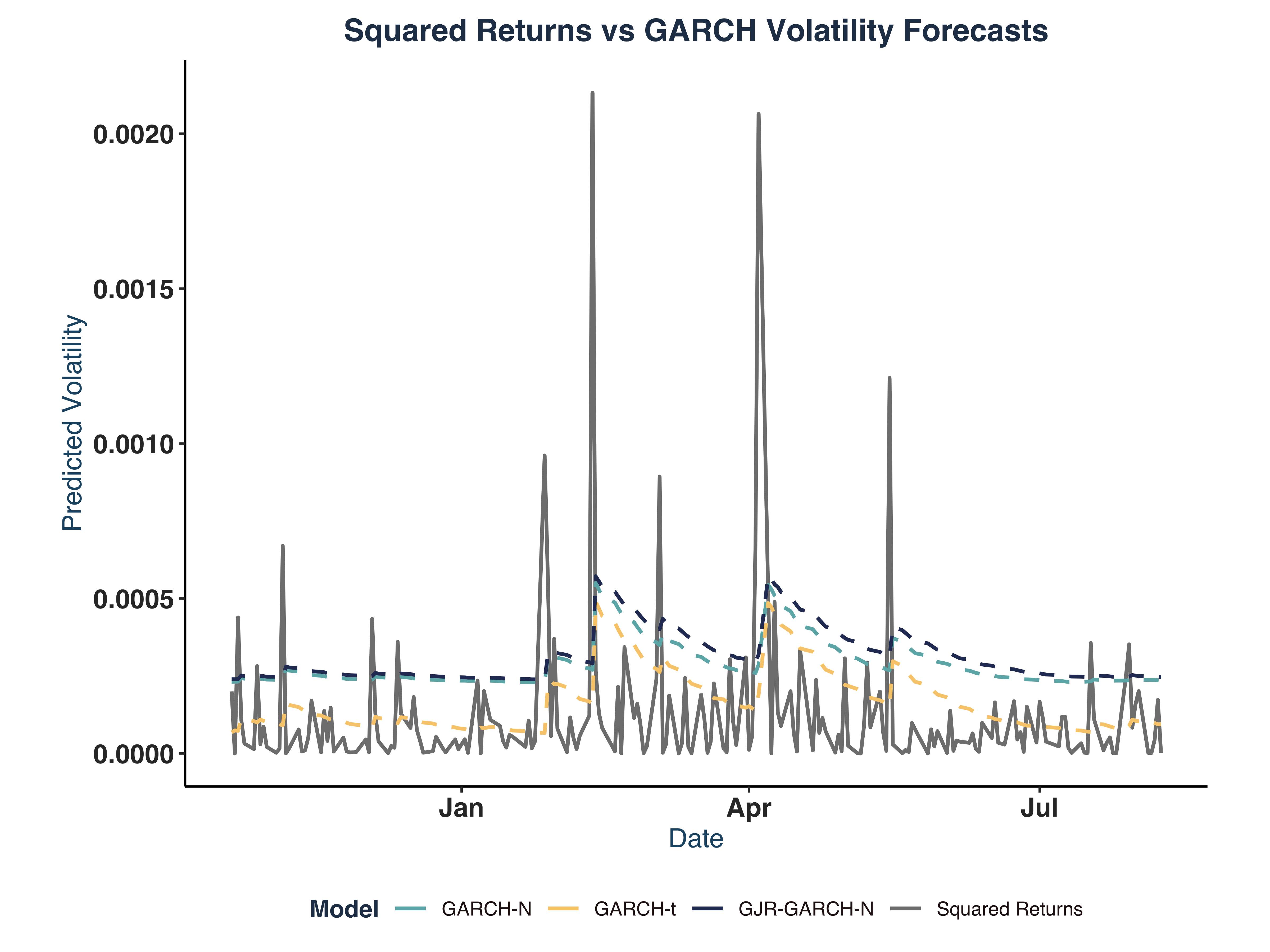
Key Findings#
1. Volatility Patterns & Market Behaviuor
- Coca-Cola demonstrates lower volatility compared to other consumer staples like Costco and Walmart, confirming its reputation as a defensive stock
- Clear volatility clustering observed across all time frequencies, with periods of high volatility followed by periods of low volatility
- Weekly and monthly returns show more pronounced volatility spikes during market stress periods, particularly evident during the 2008 financial crisis and COVID-19 pandemic
2. GARCH Model Performance
- GARCH(1,1) model effectively captures volatility dynamics with statistically significant parameters
- High persistence in volatility ($\alpha + \beta \approx 0.95-0.98$), indicating that volatility shocks have long-lasting effects
- Model successfully eliminates ARCH effects in residuals, confirming adequate specification
- Conditional volatility forecasts show realistic ranges with appropriate uncertainty bands
3. Risk-Return Profile
- Coca-Cola exhibits favorable risk-adjusted returns with relatively stable performance across different market conditions
- Annualized volatility ranges between 15-25% depending on the time period and market regime
- Lower downside risk compared to growth stocks, making it suitable for conservative portfolios
- Volatility mean-reversion properties suggest temporary spikes in uncertainty tend to normalize over time
4. Practical Investment Implications
- Coca-Cola serves as an effective portfolio diversifier due to its low correlation with market volatility during stress periods
- Predictable volatility patterns can inform options pricing and risk management strategies
- Defensive characteristics confirmed through consistent performance during market downturns
- GARCH-based volatility forecasts provide reliable inputs for portfolio optimization and Value-at-Risk calculations
5. Model Validation & Robustness
- Residual diagnostics confirm model adequacy with no remaining autocorrelation or heteroscedasticity
- Information criteria support GARCH(1,1) specification over simpler alternatives
- Out-of-sample forecasting performance demonstrates practical utility for risk management applications
- Consistent results across different return frequencies validate the robustness of findings
These findings support Coca-Cola’s classification as a low-risk, defensive investment with predictable volatility characteristics suitable for risk-averse investors and portfolio diversification strategies.
Techincal Notes#
- Analysis performed using R with tidyverse ecosystem
- Data sourced from Yahoo Finance via tidyquant
- Custom helper functions used for data preprocessing
- Visualization created with ggplot2 and ggpubr
———————————- THANK YOU ———————————-
This post is based on my S417 Mandatory Assignment for econometrics coursework at University of Tübingen.